
Examining iPhone Listings on eBay in Excel
Data Utilized
Dataset Source: UltimateAppleSamsungEcom 🍏📱💻 Dataset > iphone_ebay.csv
Purpose: This spreadsheet was created as an exercise to demonstrate potential uses for a variety of Excel formulas.
Remark. This workbook presents as a tool to be used to make informed decisions when buying an iPhone on eBay, but offers little to no real world utility due to the limitations of the underlying dataset and the intention behind this demonstration.
Workbook Overview
Tab names are in bold text.
- Listings Overview
- Simple stats:
- Price Range
- Average Price
- Median Price
- Number of Listings
- A “table” that has the columns:
- Listing Title
- Price
- Condition
- Variant
- Simple stats:
- Listing Stats
- Pivot Tables
pvtPrices- Pivot Chart:
PriceChart
- Pivot Chart:
pvtListings- Pivot Chart:
CondChart
- Pivot Chart:
- Pivot Tables
- Master-Table
- Listing Title
- Price
- Condition
- Variant
- Model (included for the pivot tables)
Named Ranges
| Title | Reference |
|---|---|
| Condition | 'Listings Overview'!$C$9 |
| iPhone13 | 'Listings Overview'!$K$17:$K$22 |
| iPhone14 | 'Listings Overview'!$L$17:$L$22 |
| iPhone15 | Listings Overview'!$M$17:$M$22 |
| Model | 'Listings Overview'!$A$4 |
| Price | 'Listings Overview'!$B$23:$B$1048576 |
| Variant | 'Listings Overview'!$B$9 |
The Contents of Each Tab
Listings Overview Tab
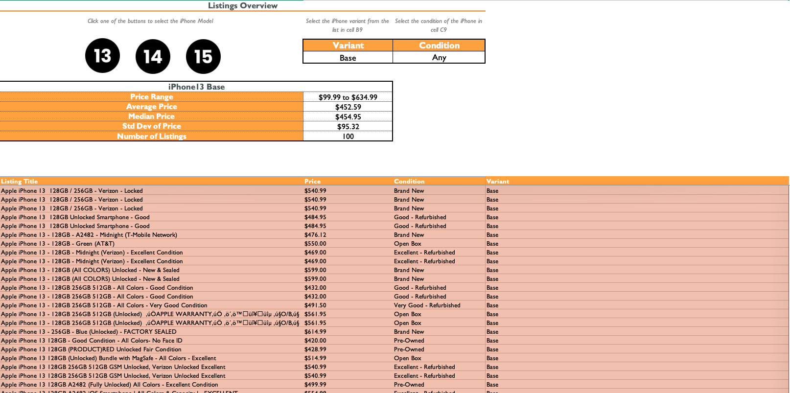
The Listings Overview tab’s purpose is to display some details about the listings included in the underlying dataset.
The user can select the iPhone model using one of the three black icons that appear in the top left. They can also select the iPhone variant and condition in cells B9 and C9 respectively.
Based on the options selected the price range, average price, median price, and number of listings values will update accordingly.
The three black icons are linked to a hidden drop-down list in cell A4 by use of macros. When clicked, the a macro will run, changing the values in the drop-down list in cell B9 (iPhone variant) accordingly.
Example.
- The black 13 icon is clicked
- The selected item in the drop-down list in
A4becomes ‘iPhone13’ which references the named range iPhone13.- The choice of variants in the drop down list in cell
B9then changes accordingly to the variants of iPhone 13s available (‘Mini’, ‘Base’ , ‘Pro’, and ‘Pro Max’).This is done with the formula
=INDIRECT($A$4)in cellB9which again, is a reference to the named range that was selected when the black icon was clicked. If the 14 icon were clicked, the choices in cellB9would change to ‘Base’, ‘Plus’, ‘Pro’, and ‘Pro Max’.
Listings Stats Tab
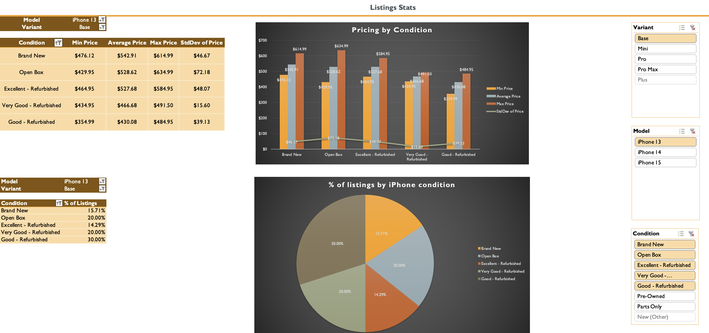
This tab contains two pivot tables, pvtPrices and pvtListings, which are each accompanied by pivot charts PriceChart and CondChart respectively.
The pivot table and pivot chart combination are both controlled by three slicers which allow the user to select which iPhone model, variant, and condition they want displayed.
pvtPricesFields
- Filters
- Model
- Variant
- Rows
- Condition
- Values
- Minimum Price
- Average Price
- Maximum Price
- Std Dev of Price
pvtListingsFields
- Filters
- Model
- Variant
- Rows
- Condition
- Values
- % of Listings
Remark. A custom list is used to sort the conditions. The “new” conditions (“Brand New”, “Open Box”) are first in ascending order, i.e. they take on the lower values.
PricesChart
This pivot chart is a cluster column chart which is linked to the pivot table pvtPrices. For each condition of phone available, it displays 3 columns on the chart for the minimum price, average price, maximum price, and standard deviation.
CondChart
This pivot chart is a pie chart which is linked to the pivot table pvtListings. Each section of the piechart corresponds to the available iPhone listing conditions. The “Condition” slicer can be used to filter which conditions appear on either chart.
Reminder: All three slicers are linked to both pivot charts.
Formula Explanations
Preliminary definitions
Named ranges are used in this spreadsheet to make formulas more readable and to create a dynamic list in cell B9 in the Listings Overview tab .
Named ranges referenced in this section :
| Title | Reference |
|---|---|
| Condition | 'Listings Overview'!$C$9 |
| iPhone13 | 'Listings Overview'!$K$17:$K$22 |
| iPhone14 | 'Listings Overview'!$L$17:$L$22 |
| iPhone15 | Listings Overview'!$M$17:$M$22 |
| Model | 'Listings Overview'!$A$4 |
| Price | 'Listings Overview'!$B$23:$B$1048576 |
| Variant | 'Listings Overview'!$B$9 |
Price - This contains the contents of column B in the Listings Overview tab
Model - (list in the hidden cell A4)
The three iPhone models included in this spreadsheet
- “iPhone13”
- “iPhone14”
- “iPhone15”
Variant - (data validation list in cell B9) * Changes based on which model is selected in cell A4
Content:
IF
A4= “iPhone13” , THENB9= {“Mini” ,”Base” , “Pro” , “Pro Max”}
IF
A4= (“iPhone14” OR “iPhone15”) , THENB9= {“Base” , “Plus”, “Pro” , “Pro Max”}
Condition (data validation list in cell C9)
Indicates what condition the iPhone is in, e.g. used or brand new. These are predefined by eBay.
Content:
“Brand New” , “New (Other)” , “Open Box”, “Excellent - Refurbished”, “Very Good - Refurbished”, “Good - Refurbished” , “Parts Only” , “Pre-Owned”
Listings Overview Tab
Drop-down lists and buttons
Example. When you click the button 13 to select the iPhone 13 model. A macro that is linked to that button selects the “iPhone13” option in the (hidden) drop-down list in
A4
In cell
B9there is a visible drop down list that contains the iPhone variantThe formula that is responsible for this drop-down list is
=INDIRECT($A$4)This drop-down list is dynamic and changes based on which iPhone model is selected in cell
A4
The stats
Below are the formulas that populate the section with basic statistics in this tab.
- Price Range:
="$"&MIN(Price)&" to $"&MAX(Price)- The
&operator concatenates the values returned byMINandMAX
- The
- Average Price:
=AVERAGE(Price) - Median Price:
=MEDIAN(Price) - Number of listings:
=COUNTA(Price)
The overview “table”
1
2
=IFS(Condition="Any", FILTER(MasterTbl[[Listing Title]:[Variant]], (SUBSTITUTE(MasterTbl[Model]," ","")=Model) * (MasterTbl[Variant]=Variant)), Condition<>"Any", FILTER(MasterTbl[[Listing Title]:[Variant]], (SUBSTITUTE(MasterTbl[Model]," ","")=Model) * (MasterTbl[Condition]=Condition) * (MasterTbl[Variant]=Variant))
)
Formula explanation: If “Any” is selected as the iPhone condition in cell C9 then the table filters listings by just the iPhone model and variant; regardless of the condition of the phone.
If any other iPhone condition is selected in C9, then the table filters by both iPhone model, variant, and condition.
Functions used: IFS, FILTER , & SUBSTITUTE
IFS formula syntax:
1
IFS(logical_test1, value_if_true1, [logical_test2, value_if_true2], [logical_test3, value_if_true3],…)
Formula breakdown:
-
Argument 1
(logical_test1): If “Any” is selected from the phone condition drop-down list in cellC9, execute Argument 2. - Argument 2
(value_if_true1)FILTER: Will return the listing name, price, condition, and variant from the tableMaterTbl(that resides in the Master-Table tab) under the conditions that the iPhone model matches the one selected with the black icons and that the variant matches the one selected in cellB9.- The
SUBSTITUTEfunction removes all spaces from the given iPhone model in column E so that it can match the formatting of theModelnamed range. - The
*operator functions as the logical operator/functionANDwithin the criteria argument in theFILTERfunction.- i.e. the row corresponding to a listing from
MasterTblis returned if and only if it has the desired model and variant.
- i.e. the row corresponding to a listing from
- The
-
Argument 3
(logical_test2): If the condition selected in cellC9is not “Any“, then execute argument 4. - Argument 4
(value_if_true2): If a listing from the tableMasterTblis of the condition that matches the one selected in cellC9and has the variant selected in cellB9, that listing is returned into the overview table.- Again, the
*operator functions as the logical operator/functionANDwithin the criteria argument in theFILTERfunction.- The row corresponding to a listing is returned if and only if it has the selected model, variant, and condition.
- Again, the
Master-Table tab
This tab was created to house the table that would act as the data source for both the Listings Overview tab and Listings Stats tabs.
It differs from the data in the iphone_ebay.csv file in that I added two columns to make the dataset more useful for my project. The columns were Variant (Column D) and Model (Column E). In the following subsections I go over the formulas that populate the cells in these two columns. I also go over the formulas I used to deal with eBay listings that were selling multiple iPhones.
The Price Column (B)
Some of the prices in the dataset were simply listed as “price ranges” in the sense that they would be in the following format : $200to$500.
In reality the listings represented that had these ranges were selling more than one storage configuration of a given iPhone model. E.g. if it is a listing for an iPhone 13 Pro Max, the listing may be selling iPhone 13 Pro Maxs at 128gb , 256gb, and 512gb of internal storage.
In that case, the minimum value of our “price range” would represent the price of the 128gb model and the maximum value of our price range would represent the price of the 512gb model. With the price of the 256gb model being unknown to us, falling somewhere between the minimum value and the maximum value.
To deal with these listings I simply took the average of the minimum and maximum value of the price range for simplicity. This unfortunately makes our data a little less reliable.
The following formula was used to return the values in the price column. The values returned were pasted as values into the price column.
Averaging of Price Ranges
1
=IFS(ISTEXT(E2),AVERAGE(NUMBERVALUE(LEFT(E2,7)),NUMBERVALUE(RIGHT(E2,7))),ISNUMBER(E2),E2)
Formula explanation: If the price is a price range (i.e. a string of text of the form $Xto$Y), it takes the average of the maximum value and minimum value. If it is simply a single numeric price it just returns that price.
Functions used: IFS, ISTEXT, AVERAGE, NUMBERVALUE, LEFT, RIGHT, and ISNUMBER
Cell E2 contains the price for the listing given by our original dataset.
Formula breakdown:
-
Argument1
ISTEXT(E2): If the price in cell E2 is a string of text (i.e. a price range), thenISTEXTwill return TRUE - Argument2
AVERAGE: If Argument1 returns TRUE then we take the average of the minimum value and maximum value of the “price range”- Both the functions
LEFTandRIGHTreturn 7 characters because an iPhone is going to be at most somewhere in the thousands of dollars. 1000.00 has 7 characters, including the decimal point. NUMBERVALUEconverts the strings extracted by theLEFTandRIGHTfunctions into the number format so thatAVERAGEcan use them in it’s calculation.
- Both the functions
- Argument3
ISNUMBER(E2), if our price is formatted as a number in Excel. I.e. it’s just a number and not a price range represented by a string of text, this argument returns the valueTRUE. - Argument4: If Argument3 is
TRUE, thenIFSsimply returns the value in cellE2.
If we had a price that was of the form $X but formatted as a number in excel then the 2nd portion of the IFS function would take the average of that single price, which would be equal to the price (i.e. there would be no change in value).
Variant (Column D)
This column’s purpose is to discern between iPhone variants of a particular model . The formula populating this column is slightly modified based on the iPhone model.
To do this, I filtered the table by model using column E and then the following formulas were used in column D.
iPhone13
1
 =IFNA(IFS(ISNUMBER(FIND("Pro Max",$A2)),"Pro Max", AND(ISNUMBER(FIND("Pro",$A2)),ISNUMBER(FIND("Pro Max",$A2))=FALSE),"Pro",ISNUMBER(FIND("Mini",$A2)),"Mini"),"Base")
iPhone14 & iPhone 15
1
=IFNA(IFS(ISNUMBER(FIND("Pro Max",A227)),"Pro Max", AND(ISNUMBER(FIND("Pro",A227)),ISNUMBER(FIND("Pro Max",A227))=FALSE),"Pro",ISNUMBER(FIND("Plus",A227)),"Plus"),"Base")
Below I provide an explanation for the iPhone13 version of this formula.
1
=IFNA(IFS(ISNUMBER(FIND("Pro Max",$A2)),"Pro Max", AND(ISNUMBER(FIND("Pro",$A2)),ISNUMBER(FIND("Pro Max",$A2))=FALSE),"Pro",ISNUMBER(FIND("Mini",$A2)),"Mini"),"Base")
Formula explanation: The basic idea is if any of the strings associated with the variants of given iPhone model are found in the listing title then the formula will return that string as the variant. e.g. If “Pro Max” is found in the listing title the formula will return “Pro Max” as the variant assuming the listing is for an iPhone 13 Pro Max Functions used: IFNA , IFS , ISNUMBER , FIND
IFNA(value, value_if_na_error)
IFS(condition1, value_if_true1, [logical_test2, value_if_true2], [logical_test3, value_if_true3],…)
Formula breakdown:
- Formula 1:
IFNA( ... , "Base")will return “Base” as the variant if none of the other strings (“Mini”, “Pro”, “Pro Max”) are found in the listing name - Formula 2
IFS:- Argument1
(logical_test1): IfFINDfinds the string “Pro Max” in the listing name (cellA2) then it returns a number marking the position of the P in “Pro Max”. In this case,ISNUMBERwill returnTRUEas the position of P will be always be a number. - Argument2
(value_if_true1): If the test is true. IFS returns “Pro Max” as the iPhone variant - Argument3
(logical_test2): If the string “Pro” is found in the listing name and it’s not a substring of “Pro Max” thenANDwill return true - Argument4
(value_if_true2): If Condition2 is true, thenIFSwill return “Pro” as the iPhone variant - Argument5
(logical_test3): IfFINDfinds the string “Mini” in the listing name (cellA2) then it returns a number marking the position of the M in “Mini”. In this case,ISNUMBERwill returnTRUEas the position of M will always be a number. - Argument6
(value_if_true3): If Condition3 is true, thenIFSwill return “Mini” as the iPhone variant.
- Argument1
Model (Column E)
Formula used in Column E (Model) : =TRIM(MID(A2,FIND("iPhone",A2),9))
Formula explanation: The formula looks for the starting point of the word “iPhone” and then prints nine characters from the starting point,. Nine characters because “iPhone 13” is nine characters long including the space. TRIM is used to remove any trailing spaces.
Example.
A2= ‘Apple iPhone 13 128GB / 256GB - Verizon - Locked’ The i in ‘iPhone’ in cellA2is the 7th character in the cell So the formula starts at position 7 and then prints nine characters starting from that position. This returns “iPhone 13” in this case.
Functions used: TRIM , MID , and FIND
Formula breakdown:
TRIM
To remove any trailing spaces from the text returned from MID and FIND
MID
Returns nine characters from cell A2, starting from the ‘i’ in ‘iPhone’
FIND
Locates the starting point of ‘iPhone’ in the cell A2
Remark. In part two of looking at this data set, I will explore price prediction models, using an updated version of this dataset.