
Predicting the Prices of Used iPhones From eBay With Python
Part 2 of Examining iPhone Listings from eBay in Excel
Data Source
The dataset iphone_ebay.csv contains scraped listings from eBay, including the product name, listed price, and condition. Below is a copy of the dataset that I utilized in this demonstration.
Here is a direct link to the kaggle page for this dataset : Dataset on Kaggle
Objective
- Clean and preprocess the raw data, extracting relevant features.
- Perform Exploratory Data Analysis (EDA) to understand data distributions and relationships.
- Build a multi-linear regression model to predict iPhone prices.
- Evaluate the model’s performance.
- Visualize key findings.
Challenges
Remark.
This dataset is quite inconsistent and lacks structure. This is a non-ideal situation but a realistic one as datasets will always require some amount of cleaning. Data that is this unstructured is not that uncommon, especially if you are crudely scraping the data yourself.Main challenges :
- Limited columns/features
- Price ranges with little insight into what they represent
- Condition is an inherently ambiguous categorical variable
We attempt our best to mitigate these challenges by:
- Extracting new features from the
namecolumn - Approximating prices from price ranges
- Mapping conditions to numbers in order to rank them
More specifically, we will create a feature iphone_full_model_variant which simply contains the iPhone model name for each listing. We will use this as one of our independet variables to predict our price as it will prove to be our best choice for a predictor variable for the purpose of prediciting iPhone prices on eBay.
Jupyter Notebook File
Below you can access a jupyter notebook file which contains the source code that will be discussed below. This is demonstrate the reproducibility of our findings.
Required Libraries
pandas: For data manipulation and analysis.numpy: For numerical operations, especially for handling arrays and mathematical functions.scikit-learn: For machine learning models (linear regression & multiple linear regression), data splitting, and evaluation metrics.seaborn: For advanced statistical data visualization.matplotlib.pyplot: For creating static, interactive, and animated visualizations.re: For regular expressions.
Problem Statement
This demonstration aims to predict the price of iPhones listed on eBay based on their model, variant (e.g. Pro & Pro Max), and condition. By leveraging machine learning techniques, we aim to understand the key factors influencing iPhone prices in the secondary market.
1. Initializing the Dataframe
1
2
3
4
5
6
7
8
9
10
11
12
13
14
15
16
17
18
19
20
21
22
23
import pandas as pd
import numpy as np
import re
import matplotlib.pyplot as plt
import seaborn as sns
from sklearn.model_selection import train_test_split
from sklearn.linear_model import LinearRegression
from sklearn.metrics import mean_absolute_error, mean_squared_error, r2_score


try:
    df = pd.read_csv('archive/iphone_ebay.csv')
    print("\nFirst 5 rows of the dataset:")
    print(df.head())
    print("\nInformation about the dataset:")
    df.info()
    print("\nDescriptive statistics of the dataset:")
    print(df.describe())
except FileNotFoundError:
    print("Error: 'iphone_ebay.csv' not found. Please ensure the file is in the correct directory.")
    exit()
1
2
3
4
5
6
7
8
9
10
11
12
13
14
15
16
17
18
19
20
21
22
23
24
25
26
27
28
29
30
31
32
33
First 5 rows of the dataset:
                                                name             price  \
0  Apple iPhone 12 Pro Max 5G - 128GB 256GB - A23...  $489.00to$529.00
1  Apple iPhone 12 - 64GB - Black (Unlocked) A217...           $435.99
2  Apple iPhone 12 Pro Max 5G A2342 - 128GB 256GB...           $579.00
3  Apple iPhone XR - 64GB - All Colors - Factory ...           $224.99
4  Apple iPhone XR 64GB Unlocked Smartphone - Ver...           $184.95

                 condition
0       Good - Refurbished
1                Brand New
2  Very Good - Refurbished
3  Very Good - Refurbished
4  Very Good - Refurbished

Information about the dataset:
<class 'pandas.core.frame.DataFrame'>
RangeIndex: 1752 entries, 0 to 1751
Data columns (total 3 columns):
 #   Column     Non-Null Count  Dtype
---  ------     --------------  -----
 0   name       1752 non-null   object
 1   price      1752 non-null   object
 2   condition  1752 non-null   object
dtypes: object(3)
memory usage: 41.2+ KB

Descriptive statistics of the dataset:
                                                     name    price  condition
count                                                1752     1752       1752
unique                                               1208      805          8
top     Apple iPhone 12 64GB Unlocked Smartphone - Ver...  $219.99  Pre-Owned
freq                                                    6       19        753
1
2
3
4
5
6
7
# Check for missing values and duplicates
print(f"\nNull values before cleaning:\n{df.isnull().sum()}")
print(f"\nNumber of duplicate rows: {df.duplicated().sum()}")

df.drop_duplicates(inplace=True)
df.reset_index(drop=True, inplace = True)
print(f"Number of rows after dropping duplicates: {len(df)}")
1
2
3
4
5
6
7
8
Null values before cleaning:
name         0
price        0
condition    0
dtype: int64

Number of duplicate rows: 531
Number of rows after dropping duplicates: 1221
We have 3 features/columns which all contain strings and zero null values.
$\approx$ 62% of our rows have unique listing names, what does that say about the nearly 30% remaining listings ?
- Some (different) sellers are using identical listing names
- Some sellers are relisting their iPhone listings on eBay because they sell numerous iPhones throughout the year
- Some sellers relist their individual iPhone until they successfully make a sale
Looking at the first 10 rows of data we can see at least one price range in our
pricefeature in dataframedf.
2. Data Cleaning and Feature Engineering
This part focuses on transforming raw data into usable features for the model, including cleaning the price, encoding the condition, and extracting iPhone model variants.
Cleaning the price column
Earlier we saw that some of the entries in price are actually price ranges. This would make any future calculations or models impossible so we will have to come up with a way to handle these ranges.
Here is how we will handle prices.
All prices
- Convert to a floating point number
Price ranges
- Take average of lower & upper bound
1
2
3
4
5
6
7
8
9
10
11
12
13
14
15
16
17
def clean_price(price_str):
    if isinstance(price_str, str):
        numbers = re.findall(r'[\d.]+', price_str.replace('$', '').replace(',', ''))
        if numbers:
            if 'to' in price_str.lower():
                if len(numbers) >= 2:
                    return (float(numbers[0]) + float(numbers[1])) / 2
            else:
                return float(numbers[0])
    return np.nan

df['price_cleaned'] = df['price'].apply(clean_price)
df.dropna(subset=['price_cleaned'], inplace=True)
df.reset_index(drop=True, inplace = True)

print(f"Rows after cleaning 'price' and dropping NaNs: {len(df)}")
df.head()
1
Rows after cleaning 'price' and dropping NaNs: 1221
| name | price | condition | price_cleaned | |
|---|---|---|---|---|
| 0 | Apple iPhone 12 Pro Max 5G - 128GB 256GB - A23... | $489.00to$529.00 | Good - Refurbished | 509.00 |
| 1 | Apple iPhone 12 - 64GB - Black (Unlocked) A217... | $435.99 | Brand New | 435.99 |
| 2 | Apple iPhone 12 Pro Max 5G A2342 - 128GB 256GB... | $579.00 | Very Good - Refurbished | 579.00 |
| 3 | Apple iPhone XR - 64GB - All Colors - Factory ... | $224.99 | Very Good - Refurbished | 224.99 |
| 4 | Apple iPhone XR 64GB Unlocked Smartphone - Ver... | $184.95 | Very Good - Refurbished | 184.95 |
Using the regular expression function findall() we retrieved all price ranges. We did this by :
- Checking to see if ‘to’ appears in the row
- Using
.lower()make sure the case of the row doesn’t cause any issues
- Using
- Then check if there is at least two matches from our row
- Take the mean of the lower and upper bound
- Or just return the single price that was retrieved
Next we will create a quantitative feature from the condition feature so that it can be incorporated into our upcoming predictive model.
1
2
3
4
5
6
7
8
9
10
11
12
13
14
15
16
17
18
19
condition_mapping = {
    'For parts or not working': 0,
    'Used - Fair': 1,
    'Used - Good': 2,
    'Pre-Owned': 2, # Assuming Pre-Owned is similar to 'Used - Good'
    'Used - Very Good': 3,
    'Good - Refurbished': 3, # Assuming Good - Refurbished is similar to 'Used - Very Good'
    'Very Good - Refurbished': 4,
    'Excellent - Refurbished': 5,
    'Brand New': 6
}

df['condition_encoded'] = df['condition'].map(condition_mapping)
df.dropna(subset=['condition_encoded'], inplace=True)
df.reset_index(drop = True, inplace = True)
df['condition_encoded'] = df['condition_encoded'].astype(int)

print(f"Rows left after encoding 'condition' and dropping NaNs: {len(df)}")
1
Rows left after encoding 'condition' and dropping NaNs: 1087
Here I mapped the all possible conditions to an integer in the range of 0 to 6. This is a system of ranking the various conditions, the higher the integer, the higher its assumed value / desirability.
I assigned the integers in our codomain to the feature condition_encoded and dropped any NaN values from the feature.
Formally, this process is referred to as ordinal encoding.
Here comes our ugliest block of code so far. Below we create the function extract_model_name() in order to create a new feature , model_name. Which we will use to create a new dataframe that has the iPhone models one-hot encoded so that we can incorporate each listings iPhone model into our upcoming predictive model.
1
2
3
4
5
6
7
8
9
10
11
12
13
14
15
16
17
18
def extract_model_name(name):
    name_lower = name.lower()
    model_match = re.search(r'(?<=iphone)\s*(xr|xs\smax|xs|x|se\s*[2-3]|se)|(([1][1-5]|[3-9])\s*(plus|pro\smax|pro|mini)?)',name_lower)
    model = model_match.group() if model_match else 'Unknown'
    return model

df['model_name'] = df['name'].apply(lambda x: pd.Series(extract_model_name(x).strip()))
df['model_name'] = df['model_name'].replace('Unknown',np.nan)
df.dropna(subset='model_name' , axis = 0)

df_processed = pd.get_dummies(df, columns = ['model_name'] , prefix='iPhone', drop_first = False)

print("\nSample of DataFrame after feature engineering:")

# Display price_cleaned next to 3 of the newly created one-hot encoded 'iPhone_' columns

sample_cols = ['price_cleaned'] + [col for col in df_processed.columns if col.startswith('iPhone')][:3]
print(df_processed[sample_cols].head())
1
2
3
4
5
6
7
Sample of DataFrame after feature engineering:
   price_cleaned  iPhone_11 pro  iPhone_11 pro max  iPhone_12
0         509.00          False              False      False
1         435.99          False              False       True
2         579.00          False              False      False
3         224.99          False              False      False
4         184.95          False              False      False
Regular expression refresher
1
r'(?<=iphone)\s*(xr|xs\smax|xs|x|se\s*[2-3]|se)|(([1][1-5]|[3-9])\s(plus|pro\smax|pro|mini)?)'
Big picture: We look for the substring 'iphone' and then search for the proceeding indicators of the various iPhone models. We either match with an X or SE model. If we find neither, then we look for indicators of other iPhone models (3,4,$\dots$, 15) (i.e. the iphone 3 to iphone 15 and their variants).
(?<=iphone)
- this code tells the machine to look for the
'iphone'substring as a “prefix” to our upcoming matches but to exclude'iphone'from our matches
(xr|xs\smax|xs|x|se\s*[2-3]|se)|(([1][1-5]|[3-9])
- We parse the listing title for the various iPhone x models , making sure to look for
'xs max'before'xs'to avoid reductively grouping all xs phones under'xs' - For SE models, we first look for 2nd or 3rd generation models, any remaining se listings will fall under
'se' - Or we look for iphone models 11 to 15 or iphone models 3 - 9 if we still don’t have a match
This leaves us with 1039 known models and 48 unknown models. You can verify this before running the lines that replace ‘Unknown’ in df['model_name'].
1
2
3
4
5
6
7
8
9
10
n_models = 0
old_models = 0

for x in df['model_name']:
    if x != 'Unknown':
        n_models += 1
    else :
        old_models += 1
        continue
print(f'We have {n_models} known models in our dataframe and {old_models} unknown models in our dataframe.')
1
2
df.reset_index(drop = True, inplace = True)
df['model_name'].value_counts()
1
2
3
4
5
6
7
8
9
10
11
12
13
14
15
16
17
18
19
20
21
22
23
24
25
26
27
28
29
30
31
32
33
34
35
36
37
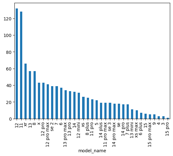
model_name
12 132
11 128
xr 66
13 57
8 57
x 43
12 pro 43
12 pro max 41
se 2 39
7 39
6 37
13 pro max 34
13 pro 33
14 32
12 mini 31
xs 26
8 plus 25
11 pro 23
5 22
14 plus 19
11 pro max 19
se 3 19
14 pro max 18
se 18
14 pro 17
7 plus 17
13 mini 11
xs max 10
6 plus 7
15 6
15 pro max 5
9 5
4 3
3 3
15 pro 1
Name: count, dtype: int64
1
2
# quick visual representation
df['model_name'].value_counts().plot.bar()
1
2
3
#number of models
model_count = len(df['model_name'].unique())
print(model_count)
1
36
Remark. I did not discern between different variants of the iPhone 3-5 as I was originally going to exclude older models entirely. While argueably lazy, very few people are actively seeking such old iPhones on the second hand market. Any model that came before the ‘plus’ variants will just be grouped under the number in the model name. e.g. The iPhone 3Gs would just fall under
iPhone_3.
3. Exploratory Data Analysis (EDA)
This section includes various visualizations to understand the distributions and relationships within the cleaned data.
First we will look at the distribution of prices amongst our cleaned price data and the listings that remain. Utilizing a histogram.
1
2
3
4
5
6
7
8
plt.figure(figsize=(10, 6))
sns.histplot(df_processed['price_cleaned'], kde=True, bins=50)
plt.title('Distribution of iPhone Prices', fontsize=16)
plt.xlabel('Price ($)', fontsize=12)
plt.ylabel('Number of Listings', fontsize=12)
plt.grid(True, linestyle='--', alpha=0.6)
plt.tight_layout()
plt.show()
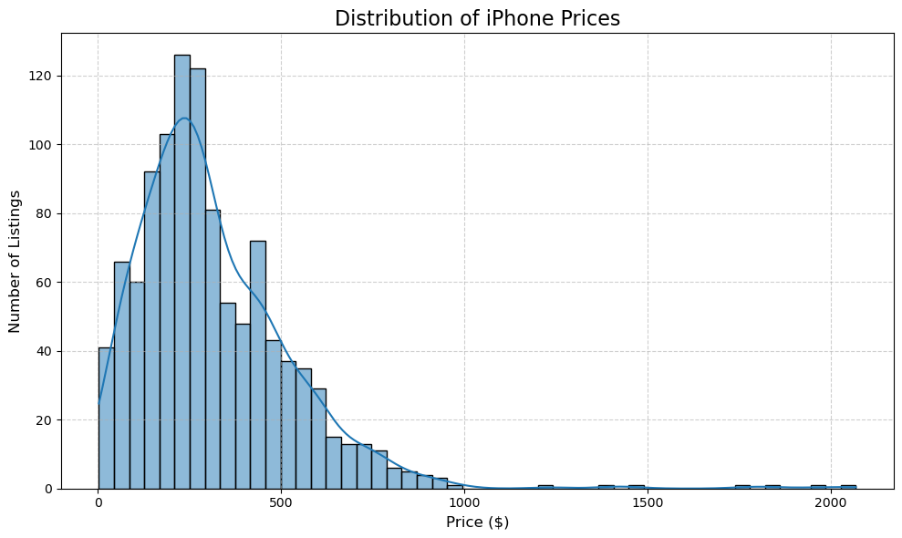
Most of our listings lie within the $[$0,$500]$ range. This is likely due to our listings being concentrated in older iPhone models such as the 11, XR, 12, 13, 8 , etc. The extremely cheap listings either fall into the “Pre-Owned” condition or are due to some sort of failure of my code to parse the listing titles effectively.
Price vs. Condition Boxplot
Here we will create a visual for the distribution of listing prices amongst the various listing conditions. Utilizing a boxplot.
1
2
3
4
5
6
7
8
9
10
11
12
13
14
15
plt.figure(figsize=(12, 7))

condition_labels = {v: k for k, v in condition_mapping.items()} #think of this as an inverse map to our conditiion_mapping map
df_for_condition_plot = df.copy()
df_for_condition_plot['condition_label'] = df_for_condition_plot['condition_encoded'].map(condition_labels) #mapping encoded output back the original condition strings , placing them in new data frame and feature
sorted_conditions = sorted(condition_mapping.keys(), key=lambda k: condition_mapping[k]) #sorting condition labels using our encoding / numerical values from the condition mapping
sns.boxplot(x='condition_label', y='price_cleaned', data=df_for_condition_plot, order=sorted_conditions, hue = 'condition_label' ,palette='viridis')
plt.title('iPhone Price Distribution by Condition', fontsize=16)
plt.xlabel('Condition', fontsize=12)
plt.ylabel('Price ($)', fontsize=12)
plt.xticks(rotation=45, ha='right', fontsize=10)
plt.yticks(fontsize=10)
plt.grid(axis='y', linestyle='--', alpha=0.6)
plt.tight_layout()
plt.show()
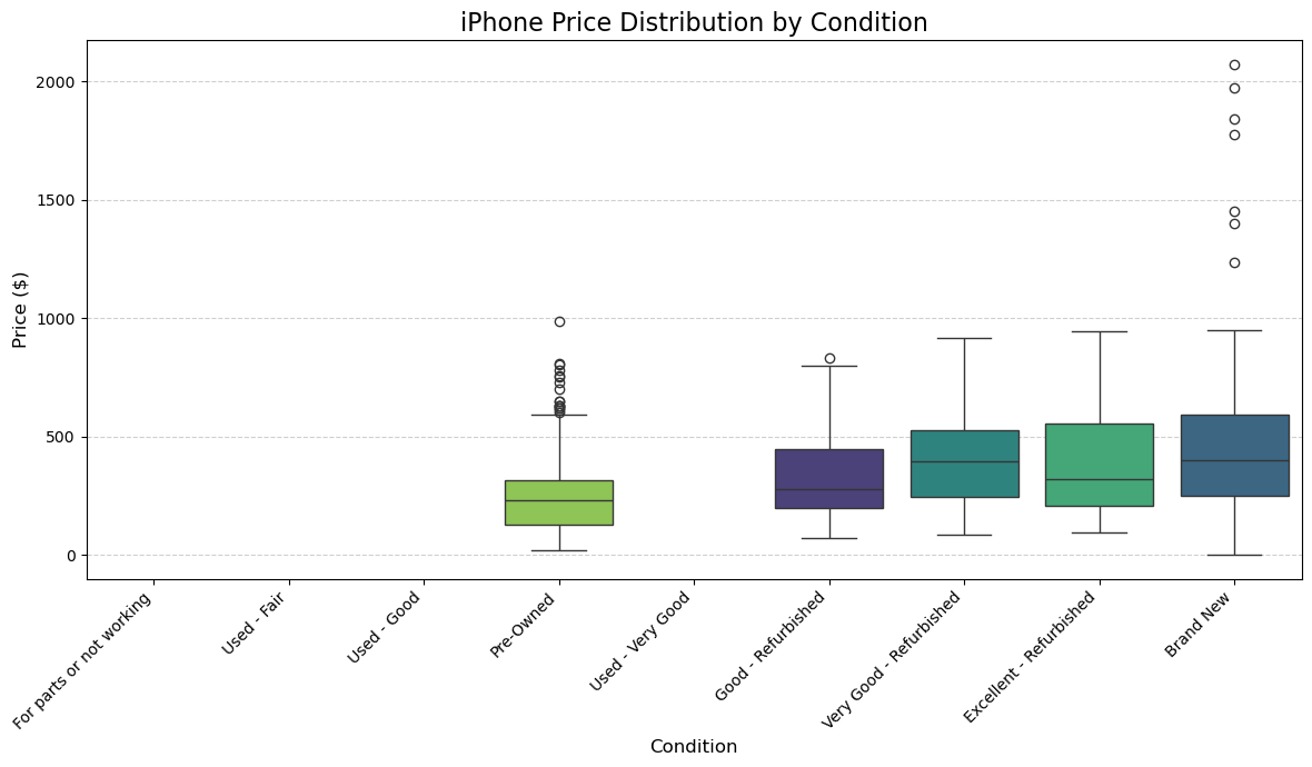
We can see that out of the remaining listings, those with “Pre-Owned” or “Brand New” condition tend to have the most outlier prices. As evidenced by all of the points above the upper extreme marker / whisker.
1
df_for_condition_plot['condition_label'].value_counts()
1
2
3
4
5
6
7
condition_label
Pre-Owned                  537
Very Good - Refurbished    166
Good - Refurbished         161
Excellent - Refurbished    113
Brand New                  110
Name: count, dtype: int64
The amount of outliers on the 'Pre-Owned' condition may be due to the shear amount of listings we have for that condition. That explanation does not really work for the 'Brand New' conditition , given that it has the least amount of listings. It is possibly due to their being less of a consensus of how to price 'Brand New' iPhones.
Next, we create a box plot to see the distribution of price amongst the top 15 iPhone models.
Distribution of Prices Across the Top 15 iPhone Models
1
2
3
4
5
6
7
8
9
10
11
12
13
14
15
16
17
18
model_counts = df['model_name'].value_counts()
top_models = model_counts.nlargest(15).sort_index().index #returns the name of the top 15 most listed models, sorted

df_top_models = df[df['model_name'].isin(top_models)].copy()


plt.figure(figsize=(14, 8))
sns.boxplot(x='model_name', y='price_cleaned', data=df_top_models, hue = 'model_name' , palette='plasma',
            order = top_models) # in order of greatest to least frequency of model
plt.title(f'iPhone Price Distribution by Top 15 Model Variants', fontsize=16)
plt.xlabel('iPhone Model Variant', fontsize=12)
plt.ylabel('Price ($)', fontsize=12)
plt.xticks(rotation=70, ha='right', fontsize=10)
plt.yticks(fontsize=10)
plt.grid(axis='y', linestyle='--', alpha=0.6)
plt.tight_layout()
#plt.savefig(fname='price-dist-by-model_boxplot')
plt.show()
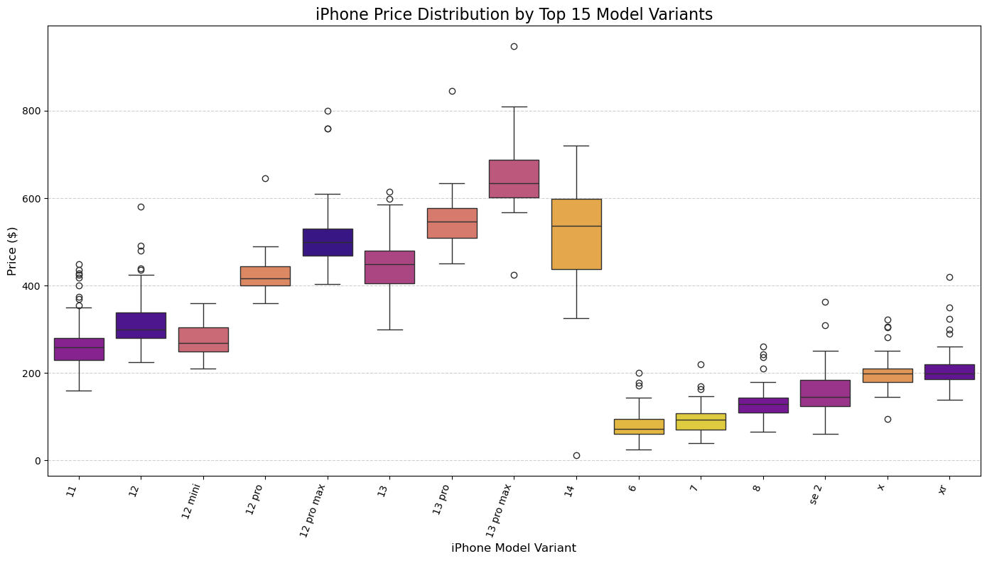
Let’s examine some of these outlier prices of our various iPhone models. Recall that an outlier is defined as a point that falls above the upper extreme or below the lower extreme in our box plot. The upper and lower extremes can be determined by the following equations.
\[\begin{align*} &\text{Upper extreme/whisker} = \text{Upper quartile} + (IQR \cdot 1.5) \\ &\text{Lower extreme/whisker} = \text{Lower quartile} - (IQR \cdot 1.5) \end{align*}\]Where $IQR$ is the interquartile range , the difference between the upper and lower quartiles.
1
2
3
4
5
6
7
8
9
10
11
12
13
14
15
cols = ['11', '8', 'xr']

for col in cols:
    df_bxmodel = df[df['model_name'] == col].copy()
    u_quart = np.percentile(df_bxmodel['price_cleaned'], 75)
    l_quart = np.percentile(df_bxmodel['price_cleaned'], 25)
    IQR = float(u_quart) - float(l_quart)
    u_extreme = u_quart + (1.5 * IQR)
    l_extreme = l_quart - (1.5 * IQR)
    outliers = [x for x in df_bxmodel['price_cleaned'] if x > u_extreme or x < l_extreme]
    print(f"\nUpper quartile value for the iPhone {col} is: {u_quart}")
    print(f"\nLower quartile value for the iPhone {col} is: {l_quart}")
    print(f"\nInterquartile range for the iPhone {col} is: {IQR}")
    print(f"\nNumber of outliers for the iPhone {col} is: {len(outliers)}")
    print("\n ---")
1
2
3
4
5
6
7
8
9
10
11
12
13
14
15
16
17
18
19
20
21
22
23
24
25
26
27
28
29
Upper quartile value for the iPhone 11 is: 279.2375

Lower quartile value for the iPhone 11 is: 229.9975

Interquartile range for the iPhone 11 is: 49.24000000000001

Number of outliers for the iPhone 11 is: 9

 ---

Upper quartile value for the iPhone 8 is: 143.6

Lower quartile value for the iPhone 8 is: 109.99

Interquartile range for the iPhone 8 is: 33.61

Number of outliers for the iPhone 8 is: 4

 ---

Upper quartile value for the iPhone xr is: 219.99

Lower quartile value for the iPhone xr is: 184.95

Interquartile range for the iPhone xr is: 35.04000000000002

Number of outliers for the iPhone xr is: 5

 ---
Here we see that out of the three selected models, the iPhone 11 (base model) has the most price outliers and the largest interquartile range.
Visualizing Correlation Data
1
2
3
4
5
6
7
8
9
10
11
correlation_features = ['price_cleaned', 'condition_encoded'] + [col for col in df_processed.columns if col.startswith('iPhone_')]
corr_matrix = df_processed[correlation_features].corr()

plt.figure(figsize=(14, 12))
sns.heatmap(corr_matrix, annot=False, cmap='coolwarm', fmt=".2f", linewidths=.5) # annot=True can make it crowded for many features
plt.title('Correlation Matrix of iPhone Models', fontsize=16)
plt.xticks(fontsize=8)
plt.yticks(fontsize=8, rotation=0)
plt.tight_layout()
plt.show()
#plt.savefig(fname = 'heatmap-modelvprice')
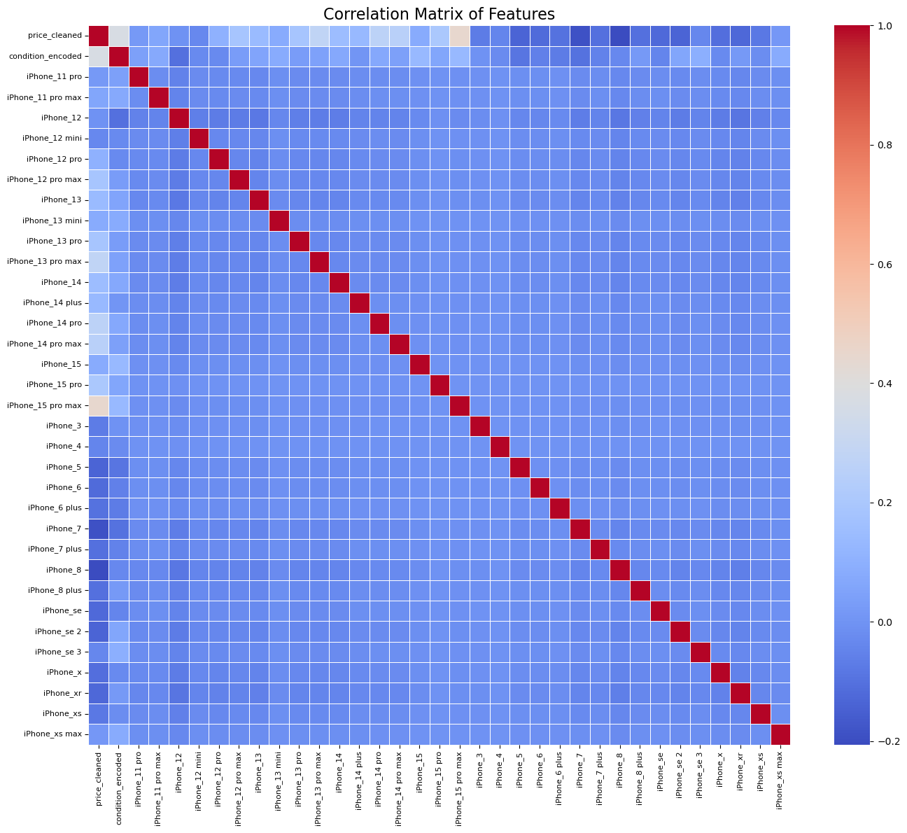
Here we can see some of the pitfalls of our dataset and the task we wished to complete with it. Some of the models with the strongest pearson correlation coefficient (in respect to price) have some of the fewest number of listings. Our wide range of model occurences in the data makes for an unbalanced and misleading correlation heatmap.
4. Model Building : Multi-Linear Regression
A model can be thought of as an equation that is used to predict a value/variable using one or more other variables. Generally we have one target / dependent variable ($y$) and at least 1 predictor/independent variable ($x_i$ where $i \geq 1$).
Target / dependent variable ($y$ or $\hat{y}$) : The variable whose value we attempt to predict with other relevant data points aka predictor variables.
Predictor / independent variables ($x_i$) : The variables used to determine the value of our target variable.
These values can not be dependent on our target, nor can they be collinear.
Collinearity in a model creates issues for a number of reasons.
- We can not be sure of the contributions of each variable to the predictions of the model
- Collinearity creates redundancy
- Collinearity results in less predictable model behavior
Coefficients in an model’s equation convey the individual contributions of our independent variables on the value of the depedent variable, holding all other variables constant. If we have collinear independent variables then neither can one be held constant if it’s also determining the value of the other to a large extent. A small change in our data may result in large changes in the value predicted by our model.
Model creation
To make use of a model we first train/fit the model on sets of training data, this how we get our parameters. In simiple linear regression (i.e. one independent variable and one dependent variable) our parameters simply are the slope of our model’s line and the y-intercept of the model. Once we have derived parameters from training, we can predict with the model.
Generally speaking a model will perform better (i.e. predict accurately and consistently) when we use relevant predictor variables.
Below we will use the iPhone model/variant and the condition of the listed iPhone as our two predictor variables. We are trying to predict the price of these iPhones, so naturally the target variable is the price. Since we have multiple predictor variables, we are using a Multi-linear regression model. Keep in mind that we have separate columns for each iphone Model/variant so we will be using upwards of 20 predictor variables.
Note: We will be using condition_encoded because a categorical variable such as condition has no way of being incorporated into our model otherwise.
Multi-linear regression
Method used to explain the relationship between:
- One continuous target $(\hat{y})$ variable
- Two or more predictor $(x_i)$ variables
Parameters
- $b_0$ : intercept
- $b_1$: coefficient of $x_1$ and so on …
1
2
3
4
5
6
7
8
9
10
11
12
13
14
15
16
17
18
19
# Define independent variables (X) and target variable (y)
# X includes condition_encoded and all one-hot encoded full_model_variant columns from df_processed

X_columns = ['condition_encoded'] + [col for col in df_processed.columns if col.startswith('iPhone_')]
X = df_processed[X_columns]
y = df_processed['price_cleaned']

# Split the data into training and testing sets
# 80% for training, 20% for testing
X_train, X_test, y_train, y_test = train_test_split(X, y, test_size=0.2, random_state=42)

print(f"Training set shape: {X_train.shape}")
print(f"Testing set shape: {X_test.shape}")

# Initialize and train the Linear Regression model
model = LinearRegression()
model.fit(X_train, y_train)

print("\nModel training complete.")
1
2
3
4
Training set shape: (869, 34)
Testing set shape: (218, 34)

Model training complete.
5. Model Evaluation
Here we will evaluate the performance of our model by calculating key statistical values and utilizing a number of visuals to aid in our evaluation.
1
2
3
4
5
6
7
8
9
10
11
y_pred = model.predict(X_test)

mae = mean_absolute_error(y_test, y_pred)
mse = mean_squared_error(y_test, y_pred)
rmse = np.sqrt(mse)
r2 = r2_score(y_test, y_pred)

print(f"Mean Absolute Error (MAE): {mae:.2f}")
print(f"Mean Squared Error (MSE): {mse:.2f}")
print(f"Root Mean Squared Error (RMSE): {rmse:.2f}")
print(f"R-squared (R2): {r2:.4f}")
1
2
3
4
Mean Absolute Error (MAE): 61.06
Mean Squared Error (MSE): 18929.33
Root Mean Squared Error (RMSE): 137.58
R-squared (R2): 0.6190
Mean Absolute Error (MAE):
\[\text{MAE} = \frac{1}{n} \sum_{i=1}^{n} |y_i - \hat{y}_i|\]Mean Squared Error (MSE):
\[\text{MSE } = \frac{1}{n} \sum_{i=1}^n (y_i - \hat{y_i})^2 \\\]Root Mean Squared Error (RMSE):
\[\text{RMSE} = \sqrt{\frac{1}{n} \sum_{i=1}^{n} (y_i - \hat{y}_i)^2}\]Variable Definitions:
- $n$: The total number of observations (data points) in the dataset.
- $y_i$: The actual (true) value of the dependent variable for the $i$-th observation.
- $\hat{y}_i$: The predicted value of the dependent variable for the $i$-th observation, determined by the iPhone model and condition.
The coefficient of determination ($R^2$):
\[R^2 = \bigg(1 - \frac{\text{MSE of regression line}}{\text{MSE of the average of the data}} \bigg)\]Actual vs Predicted iPhone Prices
1
2
3
4
5
6
7
8
9
plt.figure(figsize=(10, 6))
plt.scatter(y_test, y_pred, alpha=0.6)
plt.plot([y_test.min(), y_test.max()], [y_test.min(), y_test.max()], 'r--', lw=2) # The diagonal
plt.title('Actual vs. Predicted iPhone Prices', fontsize=16)
plt.xlabel('Actual Price ($)', fontsize=12)
plt.ylabel('Predicted Price ($)', fontsize=12)
plt.grid(True, linestyle='--', alpha=0.6)
plt.tight_layout()
plt.show()
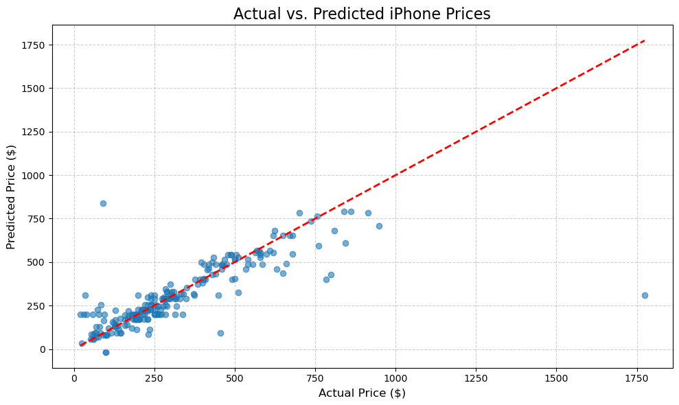
Here we can observe a lack of a strong systematic bias when looking at how the points fall above and below the diagonal. The overall slope of the scattered points appears close to the 45-degreed diagonal, indicating that the model’s scaling of predictions is reasonable.
1
2
3
4
5
6
7
8
9
residuals = y_test - y_pred
plt.figure(figsize=(10, 6))
sns.histplot(residuals, kde=True, bins=50)
plt.title('Distribution of Residuals', fontsize=16)
plt.xlabel('Residuals (Actual - Predicted Price)', fontsize=12)
plt.ylabel('Frequency', fontsize=12)
plt.grid(True, linestyle='--', alpha=0.6)
plt.tight_layout()
plt.show()
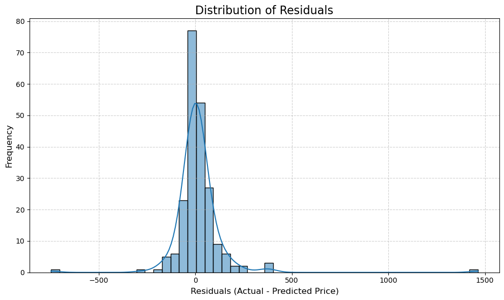
The majority of the residuals fall within a relatively narrow neighborhood around 0, meaning that most of our predictions were fairly close to the actual price values. Our residuals resemble a normal distribution, albeit with a slightly positive skewness. Our prediciton errors appear random, mirroring noise instead of having a systematic pattern to them. These are all signs that we have a linear model that performs decently well.
1
2
3
4
5
6
7
8
9
plt.figure(figsize=(10, 6))
plt.scatter(y_pred, residuals, alpha=0.6)
plt.axhline(y=0, color='r', linestyle='--', lw=2)
plt.title('Residuals vs. Predicted Prices', fontsize=16)
plt.xlabel('Predicted Price ($)', fontsize=12)
plt.ylabel('Residuals (Actual - Predicted Price)', fontsize=12)
plt.grid(True, linestyle='--', alpha=0.6)
plt.tight_layout()
plt.show()
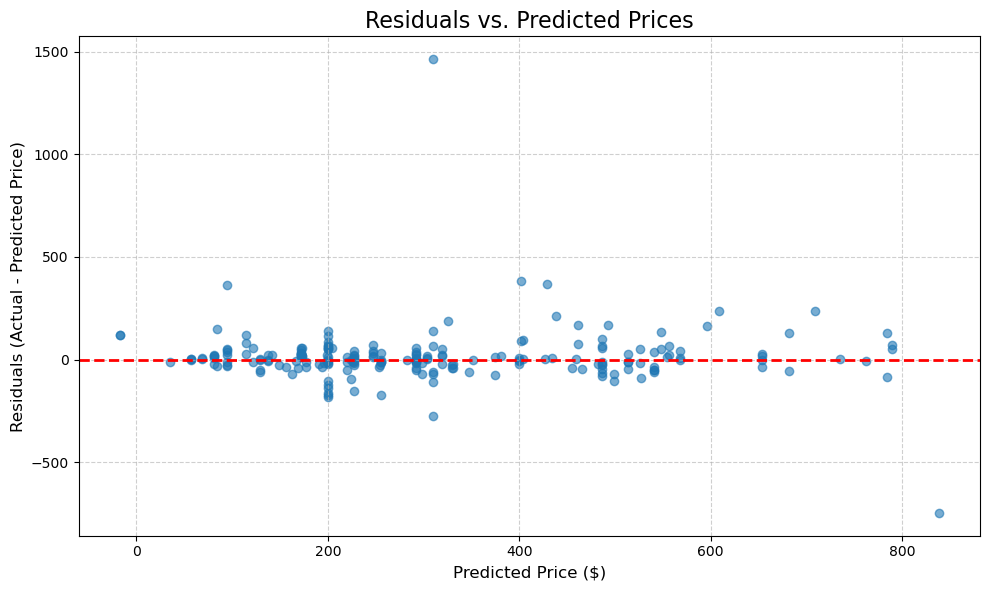
Here we can see that the residuals are mostly scattered around the horizontal line at zero. There doesn’t appear to be a significantly non-linear pattern , which likely means that the choice of a linear model (as opposed to a polynomial regression) was a good one. The variance of the errors appears to be constant, the spread of the residuals appears consistent across the domain of predicted prices. Again, this is further evidence that our model is performing decently well.
6. Conclusion
This demonstration showcased the process of bulding a multi-linear regression model to predict iPhone prices. The model acheived an $R^2$ of $0.6190$ , indicating that it explains a significant portion ($\approx 62 \%$) of the price variance. Meaning that our two chosen features make significant contributions to iPhone prices on the second hand eBay market. The Mean Absolute Error suggests that , on average , predictions are off by $ \approx $61.$ So while the model performs well relative to the other feature options, I would not use this model for anything other than a demonstration.
We can see that iPhones listed with higher encoded condition values generally cost more and that more recent iPhone models also tend to cost more. If you want to predict iPhone prices on eBay, you are better off working with relatively recent older models (anything release 2018 or later) as those appear to have the most listings to work with. Due to them being recent enough to not be considered fully deprecated, just dated at worst.
If we were to blindly go off of values of coefficients and other indicators of correlation we’d be led to believe that the newer models of iPhones are better predictors of price than older models. While this likely is true , we can not assume that with this dataset, given that only a small fraction of the listings we utilized were for iPhone 15s and 14s. E.g. $\approx 1.3 \%$ of listings were for iPhone 15s.
A model’s performance is determined by the relevance, size, and “quality” of the data that it can be trained on. If we were to collect more data and work on creating more independent features, we could generate models with higher coefficients of determination ($R^2$) and lower mean average error values.
Limitations & Potential Improvements:
- We worked with a limited number of feautres.
- Did not factor storage capacity , color, and/or battery health into our model
- Unbalanced number of listings per iPhone Model and condition
- Data is static and just a snapshot in time
- A linear model may fail to account for the complexitites of iPhone pricing
Thank you for reading through my demonstration. I hope this post was worth your time.