The Tableau Dashboard
The Jupyter Notebook
Preface
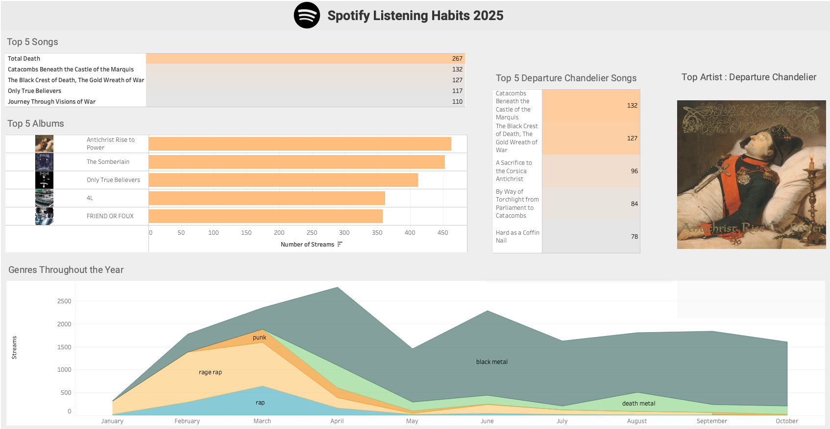
In this post I use my Spotify streaming history from 2025 to examine my listening habits. I summarized the data in a Tableau dashboard as previewed above and completed some light analysis in a Jupyter notebook.
Anyone can request their streaming history from Spotify by visiting Account Privacy under their account overview page.
The data is this post spans from Janurary 1st to October 29th.
Remark. I listen to a lot of metal. If you happen to be uncomfortable with religious or morbid themes appearing in band, album, or track names, I would not recommend reading this post. Albeit, the references to such themes in this post are rather tame.
Guiding questions
- What are my top albums of 2025?
- Who are my top artists of 2025?
- How did I interact with my top genres as the year progressed?
- What percentage of my listening is from my top artists?
- What are my top tracks from my top artist?
- What are my top artists/genres per month and season ?
- What are my busiest listening hours of the day ?
- Jupyter Lab
- Tableau
1. Create a dataframe
First, we create a loop to iterate through all of the files in our directory of Spotify data.
Note: our jupyter notebook file is in the same directory as the Spotify JSON files.
1
2
3
4
5
6
7
8
9
10
11
12
| import json
import os
import csv
import time
import datetime as dt
import calendar
import pandas as pd
import matplotlib.pyplot as plt
import seaborn as sns
import numpy as np
from spotipy.oauth2 import SpotifyOAuth
import spotipy as spot
|
1
2
3
4
5
6
7
8
9
10
11
12
13
14
15
16
17
| folder_path = "." #current directory
dfs = []
for filename in os.listdir(folder_path):
file_ext = os.path.splitext(filename)[1] #extract file extension
if file_ext == '.json':
with open (filename,'r') as f:
data = json.load(f)
dfs.append(pd.dataframe(data)) #add to the list of intermediary dataframes
else:
pass
df = pd.concat(dfs, ignore_index = True) #combines all of the dataframes in our list
df.drop("ip_addr", axis = 1 , inplace = True) # remove the IP address column
df.info()
|
1
2
3
4
5
6
7
8
9
10
11
12
13
14
15
16
17
18
19
20
21
22
23
24
25
26
27
28
29
| <class 'pandas.core.frame.dataframe'>
RangeIndex: 52451 entries, 0 to 52450
Data columns (total 22 columns):
# Column Non-Null Count Dtype
--- ------ -------------- -----
0 ts 52451 non-null object
1 platform 52451 non-null object
2 ms_played 52451 non-null int64
3 conn_country 52451 non-null object
4 master_metadata_track_name 52381 non-null object
5 master_metadata_album_artist_name 52381 non-null object
6 master_metadata_album_album_name 52381 non-null object
7 spotify_track_uri 52381 non-null object
8 episode_name 70 non-null object
9 episode_show_name 70 non-null object
10 spotify_episode_uri 70 non-null object
11 audiobook_title 0 non-null object
12 audiobook_uri 0 non-null object
13 audiobook_chapter_uri 0 non-null object
14 audiobook_chapter_title 0 non-null object
15 reason_start 52451 non-null object
16 reason_end 52451 non-null object
17 shuffle 52451 non-null bool
18 skipped 52451 non-null bool
19 offline 52451 non-null bool
20 offline_timestamp 52451 non-null int64
21 incognito_mode 52451 non-null bool
dtypes: bool(4), int64(2), object(16)
memory usage: 7.4+ MB
|
2. Dataframe modifications
We will explore the contents of our dataframe and remove any irrelevant features.
First, we set the data type for the ts (timestamp) column to datetime.
1
2
| df["ts"] = pd.to_datetime(df["ts"], utc=True)
df = df.sort_values("ts" , ignore_index=True)
|
Filter for 2025 only
1
| df = df[df["ts"].dt.year == 2025] # keep only rows where the year is 2025
|
1
2
3
4
5
6
7
| reasons = []
for x in range(0,len(data)) :
reasons.append(data[x].get("reason_end"))
reasons_set = set(reasons)
print(reasons_set)
|
1
| {'logout', 'unknown', 'trackdone', 'remote', 'unexpected-exit-while-paused', 'backbtn', 'unexpected-exit', 'fwdbtn', 'endplay'}
|
We examined a JSON file instead of the dataframe itself because the JSON file is quicker to iterate through. Most of the track-end reasons we need should be contained in every JSON file.
With the reasons in hand, we will only consider rows with 'trackdone' as its reason_end entry to count as a complete listen/stream of a track. Any other reasons will not be considered.
It seems that all rows with 'endplay' as their reason_end have True for the skipped field. The following snippet returns 8,258 rows with True and no rows with False. Therefore, we will not consider those as full streams.
1
| df.loc[(df["reason_end"] == "endplay") , "skipped"].value_counts()
|
1
2
3
| skipped
True 8258
Name: count, dtype: int64
|
Therefore we will not be considering those as full streams.
1
| df.loc[(df["reason_end"] == "trackdone" ), "skipped"].value_counts()
|
1
2
3
| skipped
False 22749
Name: count, dtype: int64
|
We edit the dataframe to only include rows with "trackdone" as the "reason_end".
1
| df = df[(df["reason_end"] == "trackdone")]
|
You can see that we went from 52,451 rows to 22,749. An approximately 56% reduction in rows.
- Amount of rows when we limit rows to (reason_end == “trackdone”) OR (reason_end == “endplay” AND skipped == False): 22,749
- Amount of rows when we limit rows to (reason_end == “trackdone”) OR (reason_end == “endplay”): 31,007
- Amount of rows when we limit to just reason_end == “trackdone”: 22,749
Rename columns
1
2
3
4
5
6
7
8
9
10
11
12
13
14
15
16
17
18
19
20
21
22
| ['ts',
'platform',
'ms_played',
'conn_country',
'master_metadata_track_name',
'master_metadata_album_artist_name',
'master_metadata_album_album_name',
'spotify_track_uri',
'episode_name',
'episode_show_name',
'spotify_episode_uri',
'audiobook_title',
'audiobook_uri',
'audiobook_chapter_uri',
'audiobook_chapter_title',
'reason_start',
'reason_end',
'shuffle',
'skipped',
'offline',
'offline_timestamp',
'incognito_mode']
|
I am really only interested in the following columns: 'ts', 'master_metadata_track_name'', 'master_metadata_album_artist_name'', 'master_metadata_album_album_name', and 'spotify_track_uri'.
I am not a fan of the columns names for artist and track information, so I will simplify them. I imagine that the "master_" prefix may be helpful for tracks that feature more than one artist, but shorter names would be easier to work with.
1
2
| master_list = [x for x in df.columns if x.startswith("master_")]
master_list
|
1
2
| for x in master_list:
df.rename(columns = {x:"_".join(x.split("_")[-2:])},inplace = True) #split feature names about the "_" delimiter and then join the last two strings in the list , with a "_" delimiter
|
Remove unneeded columns
1
2
3
4
| cols = df.columns.tolist()
cols = cols[:1] + cols[4:8]
print(cols)
df = df[cols]
|
1
| ['ts', 'track_name', 'artist_name', 'album_name', 'spotify_track_uri']
|
Update the indices on the dataframe to reflect the number of rows
1
2
| df = df.set_axis(list(range(0,len(df))), axis = 0)
df.tail()
|
| |
ts |
track_name |
artist_name |
album_name |
spotify_track_uri |
genre |
album_art_url |
season |
| 22744 |
2025-10-29 19:11:53+00:00 |
Crying for Death |
Morbid Saint |
Spectrum of Death |
spotify:track:49vQZiDk1YfTtNb04MY6jr |
thrash metal |
NaN |
Autumn |
| 22745 |
2025-10-29 19:15:01+00:00 |
Andanom |
Wulkanaz |
Wulkanaz |
spotify:track:1K2Uu3SUF5ftqxqidoLVEo |
black metal |
NaN |
Autumn |
| 22746 |
2025-10-29 19:28:49+00:00 |
Crush the Skull |
Unleashed |
Shadows in the Deep |
spotify:track:6DdtUqruR9qAaQY6IU9YG2 |
death metal |
NaN |
Autumn |
| 22747 |
2025-10-29 19:33:08+00:00 |
Bitter Loss |
Entombed |
Left Hand Path |
spotify:track:7cjxGM8tECsRdiTBYc2KFw |
death metal |
NaN |
Autumn |
| 22748 |
2025-10-29 19:36:25+00:00 |
Into Glory Ride |
Unleashed |
Where No Life Dwells |
spotify:track:7oV7uI6LsjW9dZ0iQWjyE8 |
death metal |
NaN |
Autumn |
1
2
| artist_list = list(df["artist_name"].unique())
print(f"Number of unique artists in our dataframe: {len(artist_list)}")
|
1
| Number of unique artists in our dataframe: 720
|
3. Retrieving track genres and album art (with Spotipy and the Spotify Web API)
We will create two new columns in our dataframe:
genre: contains the first listed genre for a given trackalbum_art_url: contains the url of the medium sized image of the track’s album cover.
We can fetch the data for both of these columns with the Spotify Web API, by first creating a Spotify Web App. We can make calls to the Spotify Web API using the Spotipy Python Library.
All of which you can read about here :
1
2
3
4
5
| sp = spot.Spotify(auth_manager = SpotifyOAuth(
client_id = "<CLIENT ID>",
client_secret = "<CLIENT SECRET>",
redirect_uri = "http://127.0.0.1:8081/callback"
))
|
1
| artist_list = list(df["artist_name"].unique())
|
Here search for the track information for Bitter Loss by Entombed, using it’s Spotify track URI.
1
2
| track = sp.track("spotify:track:7cjxGM8tECsRdiTBYc2KFw")
track
|
Shortened output:
1
2
3
4
5
6
7
8
9
10
11
12
13
14
15
16
17
18
19
20
21
22
23
24
25
26
27
28
29
30
31
32
33
34
35
36
37
38
39
40
41
42
43
44
45
46
47
48
49
50
51
52
53
54
55
56
57
58
59
60
61
| {'album': {'album_type': 'album',
'artists': [{'external_urls': {'spotify': 'https://open.spotify.com/artist/2pnezMcaiTHfGmgmGQjLsB'},
'href': 'https://api.spotify.com/v1/artists/2pnezMcaiTHfGmgmGQjLsB',
'id': '2pnezMcaiTHfGmgmGQjLsB',
'name': 'Entombed',
'type': 'artist',
'uri': 'spotify:artist:2pnezMcaiTHfGmgmGQjLsB'}],
'available_markets': ['AR',
'AU',
'AT',
...
'TJ',
'VE',
'ET',
'XK'],
'external_urls': {'spotify': 'https://open.spotify.com/album/5nrZejD99ZmAXrmrouIJcU'},
'href': 'https://api.spotify.com/v1/albums/5nrZejD99ZmAXrmrouIJcU',
'id': '5nrZejD99ZmAXrmrouIJcU',
'images': [{'url': 'https://i.scdn.co/image/ab67616d0000b273731794970611e9e768f5ae86',
'width': 640,
'height': 640},
{'url': 'https://i.scdn.co/image/ab67616d00001e02731794970611e9e768f5ae86',
'width': 300,
'height': 300},
{'url': 'https://i.scdn.co/image/ab67616d00004851731794970611e9e768f5ae86',
'width': 64,
'height': 64}],
'name': 'Left Hand Path',
'release_date': '1990',
'release_date_precision': 'year',
'total_tracks': 12,
'type': 'album',
'uri': 'spotify:album:5nrZejD99ZmAXrmrouIJcU'},
'artists': [{'external_urls': {'spotify': 'https://open.spotify.com/artist/2pnezMcaiTHfGmgmGQjLsB'},
'href': 'https://api.spotify.com/v1/artists/2pnezMcaiTHfGmgmGQjLsB',
'id': '2pnezMcaiTHfGmgmGQjLsB',
'name': 'Entombed',
'type': 'artist',
'uri': 'spotify:artist:2pnezMcaiTHfGmgmGQjLsB'}],
'available_markets': ['AR',
'AU',
'AT',
...
'TJ',
'VE',
'ET',
'XK'],
'disc_number': 1,
'duration_ms': 262760,
'explicit': False,
'external_ids': {'isrc': 'GBBPB0703072'},
'external_urls': {'spotify': 'https://open.spotify.com/track/7cjxGM8tECsRdiTBYc2KFw'},
'href': 'https://api.spotify.com/v1/tracks/7cjxGM8tECsRdiTBYc2KFw',
'id': '7cjxGM8tECsRdiTBYc2KFw',
'is_local': False,
'name': 'Bitter Loss',
'popularity': 31,
'preview_url': None,
'track_number': 7,
'type': 'track',
'uri': 'spotify:track:7cjxGM8tECsRdiTBYc2KFw'}
|
Notice that there is no mention of a genre in the dictionary for this track. It turns out that genres are associated with the artist and not a given track. Which is somewhat surprising, as I would have assumed it was associated with albums rather than the artists themselves. As I imagine the number of albums with disparate genres between tracks is quite low.
Let’s go about finding the first genre for each artist and add it to a new column in our dataframe called genre.
Limitations with the Spotify Web API
We have a limited number of API calls that we can make in a 30 second period, so we need to use them wisely. Here is how we will approach retrieving artist genres:
- Create a list of all artists in the dataframe.
- Iterate through the artist list.
- Find the first track in the dataframe for the artist.
- Retrieve the artist’s genres after retrieving the artist ID (by searching with the track’s URI).
- Assign the first retrieved genre to all rows for that artist.
- Repeat for the next artist in the list.
If the data I received from Spotify came with the artist IDs we could have a much simpler approach of searching for genres with the artist ID instead. At least we can use a track URI to retrieve the artist ID (as seen previously with the Entombed example).
Fetching the genres of my top 35 artists
1
2
3
| top15_artists_listens = df.artist_name.value_counts()[:15]
top15_artists_list = list(top15_artists_listens.index)
top15_artists_list
|
1
2
3
4
5
6
7
8
9
10
11
12
13
14
15
16
17
18
19
20
21
| def get_track_genres(sp, track_uri):
track = sp.track(track_uri)
artist_id = track['artists'][0]['id']
artist = sp.artist(artist_id)
genres = artist.get("genres", [])
genre = genres[0] if genres else None #return None if no Genres were retrieved
return genre
def mass_genre_fetch(sp, artist_list,df):
g_dict = dict()
for x in artist_list :
df_artist = df[df["artist_name"] == x].copy(deep = False)
if df_artist.empty:
continue
row_0 = next(df_artist.itertuples(index=False)) #we only need the first row/track
genre = get_track_genres(sp, row_0.spotify_track_uri)
df.loc[df["artist_name"] == x, "genre"] = genre #place the genre in all rows that the artist appears in
g_dict[x] = genre
return g_dict
|
Here we returned the genres of the top 15 artists and populated the df["genre"] column with their genres. We proceed to write these genres to a csv file for safekeeping.
1
2
3
4
5
6
7
8
9
10
11
12
| start = time.time()
genre_dictionary = mass_genre_fetch(sp, top15_artists_list , df)
with open("genres.csv", "w" , newline = "") as f:
writer = csv.writer(f)
writer.writerow(["Artist","Genre"])
for artist , genre in genre_dictionary.items():
writer.writerow([artist,genre])
end = time.time()
print(f"Duration of genre retrieval and csv creation: {(end - start):.2f}")
|
Looking at the CSV, Benji Blue Bills was the only artist without a genre, so I manually changed his to "rage rap".
1
| df["genre"].isnull().values.sum()
|
The approach will be to see how many artists/API calls we can get away with and try retrieving most, if not all, artist genres.
Let’s try getting the genres for the next 20 most common artists and then populate the dataframe rows for those artists with their respective genre.
1
2
| top15_to_35_artists_listens = df.artist_name.value_counts()[15:35]
top15_to_35_artists_list = list(top15_to_35_artists_listens.index)
|
1
2
3
4
5
6
7
8
9
10
11
12
| start = time.time()
genre_dictionary = mass_genre_fetch(sp, top15_to_35_artists_list , df)
with open("genres_artist_15_to_35.csv", "w" , newline = "") as f:
writer = csv.writer(f)
writer.writerow(["Artist","Genre"])
for artist , genre in genre_dictionary.items():
writer.writerow([artist,genre])
end = time.time()
print(f"Duration of genre retrieval and csv creation: {(end - start):.2f}")
|
1
| Duration of genre retrieval and csv creation: 5.31
|
That took 5.31 seconds.
Let’s find out what percentage of my streams are accounted for by my top $x$ artists (with $x$ in the range of 1 to 720 ).
1
2
| top50_artists_listens = df.artist_name.value_counts()[:50]
top50_artists_list = list(top50_artists_listens.index)
|
1
2
| top50_artists_frequency = int(df["artist_name"].isin(top50_artists_list).sum())
(top50_artists_frequency / 22749 ) * 100
|
So ≈ 70% of my streams are from my top 50 artists.
How close can we get to 100% without making the list of artists too large?
1
2
3
4
5
6
| top80_artists_listens = df.artist_name.value_counts()[:80]
top80_artists_list = list(top80_artists_listens.index)
top80_artists_list
top80_artists_frequency = int(df["artist_name"].isin(top80_artists_list).sum())
(top80_artists_frequency / len(df) ) * 100
|
1
2
| top_artists_frequency = int(df["artist_name"].isin(top_artists_list).sum())
top_artists_frequency
|
Let’s create a loop to determine what percentage of my streams are made up by my top $x$ artists. We will increment by 30 artists at a time to see how many artists are needed to cover most of the streams.
1
2
3
4
5
6
7
8
9
10
11
12
13
14
15
16
17
18
19
20
21
22
23
24
25
26
27
28
29
30
31
32
| x = 80
artists_list = list(df["artist_name"].unique())
artists_freq_list = list()
perc_of_artists_list = list() # to be used in a dataframe --> line chart , X
perc_of_listens_list = list() # to be used in a dataframe --> line chart , Y = f(X)
while x < (len(artists_list)):
top_artists_list = list(df.artist_name.value_counts()[:x].index) #top x artists from my history
artists_freq_list.append(len(top_artists_list))
top_artists_frequency = int(df["artist_name"].isin(top_artists_list).sum()) #take the sum of all occurrences of artists from top_artist_list in my dataframe
top_artists_percentage_of_listens = (top_artists_frequency / len(df) ) * 100 #the percentage of listens/streams that correspond to our current artist count
total_artists_count = len(df["artist_name"].unique())
perc_of_artists = (len(top_artists_list) / total_artists_count) * 100 #current percentage of artists being considered
perc_of_artists_list.append(perc_of_artists)
perc_of_listens_list.append(top_artists_percentage_of_listens)
print(f"{len(top_artists_list)} artists account for {top_artists_percentage_of_listens:.2f} % of my listens.\n")
print(f"{perc_of_artists:.2f}% of my artists account for {top_artists_percentage_of_listens:.2f} % of my listens.\n")
print("______________________________________")
x = x + 30
# if top_artists_percentage_of_listens >= 98.00 :
# break
# else:
# pass
Shortened output:
|
1
2
3
4
5
6
7
8
9
10
11
12
13
14
15
16
17
18
19
20
21
22
23
24
25
26
27
28
29
30
31
32
33
34
35
36
37
38
39
40
41
42
43
44
45
46
47
48
49
50
51
52
53
54
| 80 artists account for 79.21 % of my listens.
11.11% of my artists account for 79.21 % of my listens.
______________________________________
110 artists account for 84.37 % of my listens.
15.28% of my artists account for 84.37 % of my listens.
______________________________________
140 artists account for 87.84 % of my listens.
19.44% of my artists account for 87.84 % of my listens.
______________________________________
170 artists account for 90.40 % of my listens.
23.61% of my artists account for 90.40 % of my listens.
______________________________________
200 artists account for 92.28 % of my listens.
27.78% of my artists account for 92.28 % of my listens.
______________________________________
230 artists account for 93.80 % of my listens.
31.94% of my artists account for 93.80 % of my listens.
______________________________________
260 artists account for 95.02 % of my listens.
36.11% of my artists account for 95.02 % of my listens.
______________________________________
...
650 artists account for 99.69 % of my listens.
90.28% of my artists account for 99.69 % of my listens.
______________________________________
680 artists account for 99.82 % of my listens.
94.44% of my artists account for 99.82 % of my listens.
______________________________________
710 artists account for 99.96 % of my listens.
98.61% of my artists account for 99.96 % of my listens.
______________________________________
|
1
2
3
4
| plt.plot(perc_of_artists_list , perc_of_listens_list )
plt.xlabel("Percentage of Artists")
plt.ylabel("Percentage of Streams")
plt.title("% of Artists vs % of Streams")
|
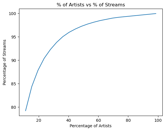
It takes the top 170 artists to cover about 90% of the streams in the 2025 Spotify history data.
Genres of my top 170 artists
1
2
3
4
5
6
7
8
9
10
11
12
13
| start = time.time()
top_35_to_170_artists_list = list(df.artist_name.value_counts()[35:170].index)
genre_dictionary = mass_genre_fetch(sp, top_35_to_170_artists_list , df)
with open("genres_artists_35_to_170.csv", "w" , newline = "") as f:
writer = csv.writer(f)
writer.writerow(["Artist","Genre"])
for artist , genre in genre_dictionary.items():
writer.writerow([artist,genre])
end = time.time()
print(f"Duration of genre retrieval and csv creation: {(end - start):.2f}")
|
1
| Duration of genre retrieval and csv creation: 32.25
|
So that took 32.25 seconds.
1
| int(df["genre"].value_counts().values.sum())
|
1
| df.to_csv("df_90perc_genres.csv", index = False)
|
Let’s save our progress to a CSV.
Manually updating genres
1
| df["genre"].value_counts()
|
1
2
3
4
5
6
7
8
9
10
11
12
13
14
15
16
17
18
19
20
21
22
23
24
25
26
27
28
29
30
31
32
33
34
35
36
37
| genre
black metal 11090
rage rap 2955
death metal 1635
rap 1227
punk 624
hardcore punk 492
jangle pop 428
melodic rap 301
dream pop 288
speed metal 226
thrash metal 209
chillwave 123
psychedelic rock 120
grunge 90
skate punk 88
underground hip hop 86
chicago drill 82
bedroom pop 51
german pop 48
shoegaze 46
indie 37
cloud rap 35
pop punk 34
riot grrrl 34
ambient folk 33
horror punk 28
neo-psychedelic 27
space rock 26
melodic death metal 25
progressive rock 24
heavy metal 23
art pop 21
brooklyn drill 20
surf rock 20
dark ambient 18
Name: count, dtype: int64
|
One of these genres doesn’t seem like something I would listen to. While it is possible, I don’t believe that I have listened to any “german pop” in 2025.
It turns out the band Greta has been categorized as “german pop”. Listen to the first 30 seconds of this song and tell me if this band sounds like they make german pop.
Spoiler: They do not. They are a 90’s grunge/hard rock band.
Greta appears to have a Spotify profile that hosts music from different artists with the same name; this likely produced the incorrect “german pop” genre for the Greta that I listen to. Notice the various faces under Greta’s discography section.

Below I have replaced “german pop” with “grunge”.
1
| df.loc[df["artist_name"] == "Greta", "genre"] = "grunge"
|
I was also suspcious of “bedroom pop”, “riot grrrl”, and “space rock”, but those genres check out and I have learned of some new genres in the process.
Below I continue to manually correct some artists’ genres.
Artists with genre values:
None: the function was unable to retrieve a genre for the artist.NaN / null: the function was not used to retrieve their genre (no attempt made).
1
2
| artists_no_genre = list(df.loc[df["genre"].isin([None]) , "artist_name"].unique())
artists_no_genre
|
1
2
3
4
5
6
7
8
9
10
11
12
13
14
| ['Young Nudy',
'Criminel Kalash',
'LAZER DIM 700',
'Nino Andretti',
'Relivelli',
'Lil Gotit',
'mizanicri',
'Peewee Longway',
'lilworld5l',
'Rio Da Yung Og',
'Jojinooo',
'KrispyLife Kidd',
'Akvan',
'Aria']
|
1
2
| df.loc[df["artist_name"] == "Young Nudy","genre"] = "rap"
df.loc[df["artist_name"] == "Young Nudy" ,"genre"]
|
1
2
3
4
5
6
7
8
9
10
11
12
| 1 rap
465 rap
466 rap
467 rap
468 rap
...
15537 rap
15682 rap
15733 rap
16563 rap
20040 rap
Name: genre, Length: 416, dtype: object
|
1
2
3
4
| index_rap = [1,2,5,7,9,11]
rap_artists_none_genre = list()
for x in index_rap :
rap_artists_none_genre.append(artists_no_genre[x])
|
1
2
| df.loc[df["artist_name"].isin(rap_artists_none_genre),"genre"] = "rap"
df.loc[df["artist_name"].isin(rap_artists_none_genre)]
|
1
2
| df.loc[df["artist_name"] == "Akvan","genre"] = "black metal"
df.loc[df["artist_name"] == "Aria","genre"] = "heavy metal"
|
1
2
| artists_no_genre = list(df.loc[df["genre"].isin([None]) , "artist_name"].unique())
artists_no_genre
|
1
| ['Criminel Kalash', 'Jojinooo']
|
1
| df.loc[df["artist_name"].isin(artists_no_genre),"genre"] = "rap"
|
1
2
| artists_no_genre = list(df.loc[df["genre"].isin([None]) , "artist_name"].unique())
artists_no_genre
|
Export another dictionary with all artists and their genres
1
| df["genre"].value_counts()
|
1
2
3
4
5
6
7
8
9
10
11
12
13
14
15
16
17
18
19
20
21
22
23
24
25
26
27
28
29
30
31
32
33
34
35
36
| genre
black metal 11090
rage rap 2955
death metal 1635
rap 1227
punk 624
hardcore punk 492
jangle pop 428
melodic rap 301
dream pop 288
speed metal 226
thrash metal 209
chillwave 123
psychedelic rock 120
skate punk 88
underground hip hop 86
chicago drill 82
bedroom pop 51
shoegaze 46
grunge 42
indie 37
cloud rap 35
riot grrrl 34
pop punk 34
ambient folk 33
horror punk 28
neo-psychedelic 27
space rock 26
melodic death metal 25
progressive rock 24
heavy metal 23
art pop 21
brooklyn drill 20
surf rock 20
dark ambient 18
Name: count, dtype: int64
|
1
2
3
4
| genres_dict_90perc = dict()
artists_w_genre_list = list(df.loc[df["genre"].isnull() == False ,"artist_name"].unique())
artists_w_genre_list
len(artists_w_genre_list)
|
1
2
| artists = df["artist_name"].unique()
len(artists)
|
1
2
| artists_wo_genre_list = list(df.loc[df["genre"].isnull(),"artist_name"].unique())
len(artists_wo_genre_list)
|
This adds up given that we only attempted to retrieve the genres for the first 170 most listened to artists. We have 720 artists in our dataframe, and 550 of them have a null value for their genre. Let’s export our completed list of the 170 artists’ genres into a CSV.
1
2
3
4
5
6
| genres_dict_top170 = dict()
for x in artists_w_genre_list:
genres_dict_top170[x] = list(df.loc[df["artist_name"] == x , "genre"].unique())[0]
len(genres_dict_top170)
|
1
2
3
4
5
| with open("genres_artists_top170.csv", "w" , newline = "") as f:
writer = csv.writer(f)
writer.writerow(["Artist","Genre"])
for artist , genre in genres_dict_top170.items():
writer.writerow([artist,genre])
|
Fetching the album art for my top 20 albums of 2025
Let’s get album art URLs for my top 20 albums before fetching any more genres. According to the Spotipy documentation, each album has cover art URLs in multiple sizes; the images are ordered from largest to smallest, so larger indices correspond to smaller images. Here are the two functions that we will use for album art retrieval. They are very similar to the genre fetching functions.
1
2
3
4
5
6
7
8
| def get_album_art(sp, track_uri):
track = sp.track(track_uri)
image_urls = track["album"]["images"]
if len(image_urls) >= 2 :
album_art_url = image_urls[-2]["url"] # 2nd to smallest size
else:
album_art_url = image_urls[0]["url"]
return album_art_url
|
1
2
3
4
5
6
7
8
9
10
11
| def mass_album_art_fetch(sp, album_list,df):
"""Retrieves url for album art, stores in dataframe, returns dictionary of album art urls"""
album_dict = dict()
for x in album_list :
df_albums = df[df["album_name"] == x ]
row_0 = next(df_albums.itertuples(index=False))
album_art_url = get_album_art(sp, row_0.spotify_track_uri)
df.loc[df["album_name"] == x, "album_art_url"] = album_art_url #place the genre in all rows that the artist appears in
album_dict[x] = album_art_url
return album_dict
|
Let’s test the first one out on a song.
1
2
| what_we_started_art = get_album_art(sp,'spotify:track:3zB4cvjs2sJ6FrBmfVZB1v')
what_we_started_art
|
1
| 'https://i.scdn.co/image/ab67616d00001e02667db8ddb394b4abeac73549'
|

Looks like it works. Let’s proceed to my top 20 albums.
1
2
3
4
| #albums_dict = mass_album_art_fetch(sp, top10_albums , df)
top20_albums_listens = df.album_name.value_counts().nlargest(20)
top20_albums_listens
top20_albums = list(top20_albums_listens.index)
|
1
2
3
4
| start = time.time()
albums_dict = mass_album_art_fetch(sp, top20_albums , df)
end = time.time()
print(f"Top 20 Album covers fetched in :{end - start:.2f} seconds")
|
1
| Top 20 Album covers fetched in :2.97 seconds
|
Similar to what we did with artists, let’s see what percentage of my streams my $x$ top albums account for.
1
2
3
4
5
6
7
8
9
10
11
12
13
14
15
16
17
18
19
20
21
22
23
24
25
26
| x = 20
albums_list = list(df["album_name"].unique())
albums_freq_list = list()
perc_of_albums_list = list() # to be used in a dataframe --> plot , X
perc_of_listens_by_albums_list = list() # to be used in a dataframe --> line chart , Y = f(X)
while x < (len(albums_list)):
top_albums_list = list(df.album_name.value_counts()[:x].index)
albums_freq_list.append(len(top_albums_list))
top_albums_frequency = int(df["album_name"].isin(top_albums_list).sum()) #the total quantity of times our current selection of albums (quantity = x) appear in our dataframe
top_albums_percentage = (top_albums_frequency / len(df) ) * 100 #percentage of total listens/streams that corresponds to our current album count (x)
total_albums_count = len(df["album_name"].unique())
perc_of_albums = (len(top_albums_list) / total_albums_count) * 100 #current percentage of albums
perc_of_albums_list.append(perc_of_albums)
perc_of_listens_by_albums_list.append(top_albums_percentage) # the list of percentages of total streams that correspond to each given quantity of albums (x)
print(f"{len(top_albums_list)} albums account for {top_albums_percentage:.2f} % of my listens.\n")
print(f"{perc_of_albums:.2f}% of my albums account for {top_albums_percentage:.2f} % of my listens.\n")
print("______________________________________")
x = x + 20
if top_albums_percentage >= 99.00 :
break
|
Shortened output:
1
2
3
4
5
6
7
8
9
10
11
12
13
14
15
16
17
18
19
20
21
22
23
24
25
26
27
28
29
30
| 20 albums account for 26.02 % of my listens.
1.48% of my albums account for 26.02 % of my listens.
______________________________________
40 albums account for 40.90 % of my listens.
2.97% of my albums account for 40.90 % of my listens.
______________________________________
60 albums account for 50.90 % of my listens.
4.45% of my albums account for 50.90 % of my listens.
______________________________________
80 albums account for 58.05 % of my listens.
5.93% of my albums account for 58.05 % of my listens.
...
______________________________________
1120 albums account for 98.99 % of my listens.
83.02% of my albums account for 98.99 % of my listens.
______________________________________
1140 albums account for 99.08 % of my listens.
84.51% of my albums account for 99.08 % of my listens.
______________________________________ ...
|
1
2
3
4
| plt.plot(perc_of_albums_list ,perc_of_listens_by_albums_list )
plt.xlabel("Percentage of Total Albums")
plt.ylabel("Percentage of Streams")
plt.title("% of Albums vs % of Streams")
|
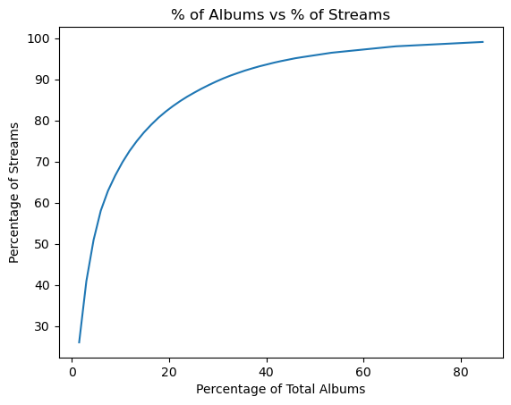
Another logarithmic curve, we only need to retrieve a fraction of the top albums’ cover art in order to retrieve the album art for most of my streams. But my main motivation for fetching album art is to have some visuals for our dashboard. So I am satisfied with only fetching the cover art for the top 20 albums.
1
| df.to_csv("df_ninety_perc_genres.csv", index = False)
|
Write our progress to another csv.
Processing dates: season feature
We will create a season feature for the dataframe.
1
2
3
4
5
6
7
8
9
10
11
12
13
| def get_season(date):
date_str = str(date)[:10] #to omit the time
date_no_time = dt.datetime.strptime(date_str, "%Y-%m-%d")
month = date_no_time.month
if month in [12,1,2]:
return "Winter"
elif month in [3,4,5]:
return "Spring"
elif month in [6,7,8]:
return "Summer"
elif month in [9,10,11]:
return "Autumn"
|
1
| df["season"] = df["ts"].apply(get_season)
|
1
| df = pd.read_csv('df_ninety_perc_genres_top20_albums.csv')
|
1
| df.to_csv("df_90perc_genres_top20_albums_seasons.csv", index = False)
|
Fetching the remaining genres
I plan to fetch genres for as many of the remaining artists as possible. I’m comfortable missing genres for around 5% of streams, so I’ll attempt to retrieve genres for the top 260 artists (which earlier analysis showed accounts for about 95% of listens).
1
2
3
4
5
6
7
8
9
10
11
12
13
| start = time.time()
top_170_to_260_artists_list = list(df.artist_name.value_counts()[170: 260].index)
genre_dictionary_170_to_260 = mass_genre_fetch(sp, top_170_to_260_artists_list ,df)
with open("genres_artists_170_to_260.csv", "w" , newline = "") as f:
writer = csv.writer(f)
writer.writerow(["Artist","Genre"])
for artist , genre in genre_dictionary_170_to_260.items():
writer.writerow([artist,genre])
end = time.time()
print(f"Duration of genre retrieval and csv creation: {(end - start):.2f}")
|
1
| Duration of genre retrieval and csv creation: 24.24
|
1
| df["genre"].isnull().value_counts()
|
1
2
3
4
| genre
False 21379
True 1370
Name: count, dtype: int64
|
So around 6.4% of rows have no genre. For this project that is acceptable.
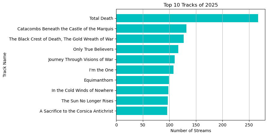
Remark. While working on the Tableau dashboard, I realized that one of our top three songs didn’t have a URL for its album art. So I fetched it manually.
1
| df.loc[df["album_name"] == "The Black Crest of Death, The Gold Wreath of War" , "album_art_url"] = get_album_art(sp,'spotify:track:44ps4XL3yOHNYguUe80yB0')
|
1
2
| bcd_gww = get_album_art(sp,'spotify:track:44ps4XL3yOHNYguUe80yB0')
bcd_gww
|
1
| 'https://i.scdn.co/image/ab67616d00001e027576cbb23bb611e042408722'
|

1
| df.loc[df["album_name"] == "The Black Crest of Death, The Gold Wreath of War" , "album_art_url"]
|
1
2
3
4
5
6
7
8
9
10
11
12
| 8927 https://i.scdn.co/image/ab67616d00001e027576cb...
8928 https://i.scdn.co/image/ab67616d00001e027576cb...
8929 https://i.scdn.co/image/ab67616d00001e027576cb...
8933 https://i.scdn.co/image/ab67616d00001e027576cb...
9018 https://i.scdn.co/image/ab67616d00001e027576cb...
...
21804 https://i.scdn.co/image/ab67616d00001e027576cb...
22075 https://i.scdn.co/image/ab67616d00001e027576cb...
22076 https://i.scdn.co/image/ab67616d00001e027576cb...
22077 https://i.scdn.co/image/ab67616d00001e027576cb...
22407 https://i.scdn.co/image/ab67616d00001e027576cb...
Name: album_art_url, Length: 193, dtype: object
|
Let’s save another copy of our dataframe to a CSV file.
1
2
| df.to_csv("df_95perc_genres_top20_albums_seasons.csv", index = False)
df.info()
|
1
2
3
4
5
6
7
8
9
10
11
12
13
14
15
| <class 'pandas.core.frame.dataframe'>
RangeIndex: 22749 entries, 0 to 22748
Data columns (total 8 columns):
# Column Non-Null Count Dtype
--- ------ -------------- -----
0 ts 22749 non-null datetime64[ns, UTC]
1 track_name 22748 non-null object
2 artist_name 22748 non-null object
3 album_name 22748 non-null object
4 spotify_track_uri 22748 non-null object
5 genre 21379 non-null object
6 album_art_url 6113 non-null object
7 season 22749 non-null object
dtypes: datetime64[ns, UTC](1), object(7)
memory usage: 1.4+ MB
|
When creating the Tablueau dashboard, we simply import the latest copy of our csv for our dashboard’s dataset.
4. Exploratory data analysis
Let’s create some simple charts in Python to learn more about my listening habits.
Genres pie chart
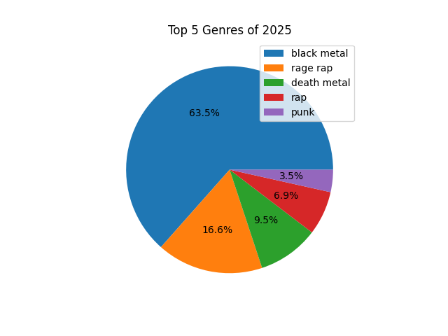
I am curious to see my top five music genres, and the percentage of my streams that belong to each.
1
2
3
4
5
6
7
8
9
| pie = df['genre'].value_counts().nlargest(5).plot(
kind='pie',
autopct='%1.1f%%',
legend=True,
labels=None
)
plt.title('Top 5 Genres of 2025')
plt.ylabel('')
plt.show()
|
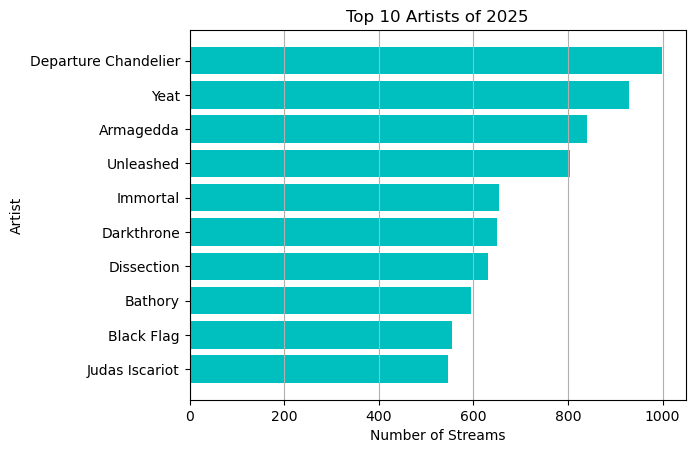
Top 10 artists
Here we create a horizontal bar chart for the top 10 artists, ranking them by number of listens/streams.
1
2
| top10_artists_listens = df.artist_name.value_counts().nlargest(10)
top10_artists = top10_artists_listens.index
|
1
2
3
| Index(['Departure Chandelier', 'Yeat', 'Armagedda', 'Unleashed', 'Immortal',
'Darkthrone', 'Dissection', 'Bathory', 'Black Flag', 'Judas Iscariot'],
dtype='object', name='artist_name')
|
1
2
3
4
5
6
7
| plt.barh(top10_artists, width = top10_artists_listens , color = 'c' , align = 'center')
plt.grid(axis = "x")
plt.xlabel("Number of Streams")
plt.ylabel("Artist")
plt.title("Top 10 Artists of 2025")
plt.gca().invert_yaxis()
plt.show()
|
Alternatively, we could have used
1
2
3
4
5
6
7
8
9
10
11
| top_artists = df["artist_name"].value_counts().nlargest(10)
ax = top_artists.plot(
kind="barh",
title="Top 10 artists",
xlabel="Number of streams",
ylabel="Artist",
color="c"
)
ax.grid(axis="x")
ax.invert_yaxis()
|
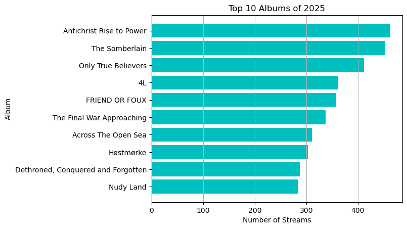
Top 10 albums
1
2
| top10_albums_listens = df.album_name.value_counts().nlargest(10)
top10_albums = top10_albums_listens.index
|
1
2
3
4
5
6
7
| plt.barh(top10_albums, width = top10_albums_listens , color = 'c' )
plt.grid(axis = "x")
plt.xlabel("Number of Streams")
plt.ylabel("Album")
plt.title("Top 10 Albums of 2025")
plt.gca().invert_yaxis()
plt.show()
|
Top 10 tracks
1
2
| top10_track_listens = df["track_name"].value_counts().nlargest(10)
top10_tracks = top10_track_listens.index
|
1
2
3
4
5
6
7
| plt.barh(top10_tracks , width = top10_track_listens , color = "c" , align = "center")
plt.grid(axis = "x")
plt.gca().invert_yaxis()
plt.title("Top 10 Tracks of 2025")
plt.xlabel("Number of Streams")
plt.ylabel("Track Name")
plt.show()
|
Finding the top artist or genre for the month or season
Finding the top artist for each month:
1
2
3
4
5
6
7
8
9
| months = list(calendar.month_name[1:11])
artists_month = dict()
for x,y in zip(range(1,11) ,months):
top_artist = df.loc[df["ts"].dt.month == x , "artist_name"].value_counts().idxmax()
artists_month[y] = top_artist
artists_month
|
1
2
3
4
5
6
7
8
9
10
| {'January': 'Yeat',
'February': 'Yeat',
'March': 'Young Thug',
'April': 'Unleashed',
'May': 'Unleashed',
'June': 'Departure Chandelier',
'July': 'Armagedda',
'August': 'Armagedda',
'September': 'Wagner Ödegård',
'October': 'Wagner Ödegård'}
|
1
2
| df_months = pd.dataframe.from_dict(artists_month , orient="Index", columns= ["top_artist"])
df_months
|
| |
top_artist |
| January |
Yeat |
| February |
Yeat |
| March |
Young Thug |
| April |
Unleashed |
| May |
Unleashed |
| June |
Departure Chandelier |
| July |
Armagedda |
| August |
Armagedda |
| September |
Wagner Ödegård |
| October |
Wagner Ödegård |
1
| df_months.to_csv("df_top_artist_per_month.csv")
|
Finding the top artist for each season:
1
2
3
4
5
6
7
8
| seasons = ["Winter","Spring", "Summer","Autumn"]
artist_per_season = dict()
for x in seasons:
season_artist = df.loc[df["season"] == x , "artist_name"].value_counts().idxmax()
artist_per_season[x] = season_artist
artist_per_season
|
1
2
3
4
| {'Winter': 'Yeat',
'Spring': 'Unleashed',
'Summer': 'Armagedda',
'Autumn': 'Wagner Ödegård'}
|
Finding the top genre for each season:
1
2
3
4
5
6
7
| genre_per_season = dict()
for x in seasons:
season_genre = df.loc[df["season"] == x , "genre"].value_counts().idxmax()
genre_per_season[x] = season_genre
genre_per_season
|
1
2
3
4
| {'Winter': 'rage rap',
'Spring': 'black metal',
'Summer': 'black metal',
'Autumn': 'black metal'}
|
Finding the busiest hours of the day
We will find the busiest streaming hours of each day and find the average peak streaming hour for each month. I.e. during what hour (in a 24 hour period) do I stream the most songs in a given day ?
First we’ll create a new dataframe with the following columns:
- “ts” : timestamp (imported from
df).
- “day_ind” : short for day index .
- “hour_ind” : short for hour index .
- “month” : corresponding to the month’s number (e.g. October and 10).
- “month_name” : the month’s name.
- “busiest_hour” : the hour with the most streams for a given day.
1
2
3
4
5
6
7
8
9
10
| df_days_hours = df.copy()
df_days_hours["day_ind"] = df_days_hours["ts"].dt.day_of_year
df_days_hours["hour_ind"] = df_days_hours["ts"].dt.hour
df_days_hours["month"] = df_days_hours["ts"].dt.month
cols_list = df_days_hours.columns.tolist()
cols = cols_list[:1] + cols_list[8:11]
df_days_hours = df_days_hours[cols]
df_days_hours
|
| |
ts |
day_ind |
hour_ind |
month |
| 0 |
2025-01-01 02:27:17+00:00 |
1 |
2 |
1 |
| 1 |
2025-01-01 02:30:24+00:00 |
1 |
2 |
1 |
| 2 |
2025-01-01 02:32:29+00:00 |
1 |
2 |
1 |
| 3 |
2025-01-01 02:34:07+00:00 |
1 |
2 |
1 |
| 4 |
2025-01-01 02:35:35+00:00 |
1 |
2 |
1 |
| … |
… |
… |
… |
… |
| 22744 |
2025-10-29 19:11:53+00:00 |
302 |
19 |
10 |
| 22745 |
2025-10-29 19:15:01+00:00 |
302 |
19 |
10 |
| 22746 |
2025-10-29 19:28:49+00:00 |
302 |
19 |
10 |
| 22747 |
2025-10-29 19:33:08+00:00 |
302 |
19 |
10 |
| 22748 |
2025-10-29 19:36:25+00:00 |
302 |
19 |
10 |
22749 rows × 4 columns
Create the month_name feature:
1
2
3
4
| for x in df_days_hours["month"]:
df_days_hours.loc[df_days_hours["month"] == int(x) ,"month_name"] = calendar.month_name[x]
df_days_hours.tail()
|
| |
ts |
day_ind |
hour_ind |
month |
month_name |
| 22744 |
2025-10-29 19:11:53+00:00 |
302 |
19 |
10 |
October |
| 22745 |
2025-10-29 19:15:01+00:00 |
302 |
19 |
10 |
October |
| 22746 |
2025-10-29 19:28:49+00:00 |
302 |
19 |
10 |
October |
| 22747 |
2025-10-29 19:33:08+00:00 |
302 |
19 |
10 |
October |
| 22748 |
2025-10-29 19:36:25+00:00 |
302 |
19 |
10 |
October |
We have up to 302 days in our dataframe, we will use that info when determining the busiest hour of the day.
1
2
3
4
5
6
7
8
9
10
| df_busiest_hour = df_days_hours.copy()
days_list = list(range(1,303)) # since we have 302 days in df & df_days_hours
for x in days_list :
if len(df_days_hours.loc[df_days_hours["day_ind"] == int(x) , "hour_ind"].value_counts()) > 0 : #if the array of value_counts is non-empty
max_hour = df_days_hours.loc[df_days_hours["day_ind"] == int(x) , "hour_ind"].value_counts().idxmax() #retrieve the max hour
df_days_hours.loc[df_days_hours["day_ind"] == int(x) , "busiest_hour"] = int(max_hour)
else:
df_days_hours.loc[df_days_hours["day_ind"] == int(x) , "busiest_hour"] = None #assign none if the value_counts series is empty
|
Let’s see if the busiest hour for day 1 being 10.0 checks out.
1
| df_days_hours.loc[df_days_hours["day_ind"] == 1]
|
| |
ts |
day_ind |
hour_ind |
month |
month_name |
busiest_hour |
| 0 |
2025-01-01 02:27:17+00:00 |
1 |
2 |
1 |
January |
10.0 |
| 1 |
2025-01-01 02:30:24+00:00 |
1 |
2 |
1 |
January |
10.0 |
| 2 |
2025-01-01 02:32:29+00:00 |
1 |
2 |
1 |
January |
10.0 |
| 3 |
2025-01-01 02:34:07+00:00 |
1 |
2 |
1 |
January |
10.0 |
| 4 |
2025-01-01 02:35:35+00:00 |
1 |
2 |
1 |
January |
10.0 |
| … |
… |
… |
… |
… |
… |
… |
| 86 |
2025-01-01 23:53:06+00:00 |
1 |
23 |
1 |
January |
10.0 |
| 87 |
2025-01-01 23:55:22+00:00 |
1 |
23 |
1 |
January |
10.0 |
| 88 |
2025-01-01 23:57:20+00:00 |
1 |
23 |
1 |
January |
10.0 |
| 89 |
2025-01-01 23:58:29+00:00 |
1 |
23 |
1 |
January |
10.0 |
| 90 |
2025-01-01 23:59:42+00:00 |
1 |
23 |
1 |
January |
10.0 |
1
| df_days_hours.loc[df_days_hours["day_ind"] == 1, "hour_ind"].value_counts()
|
1
2
3
4
5
6
7
8
9
10
11
| hour_ind
10 25
12 17
9 12
11 10
23 10
13 7
2 6
4 3
20 1
Name: count, dtype: int64
|
1
2
3
4
| df_busiest_hours = df_days_hours[["day_ind" ,"month_name" ,"busiest_hour"]]
df_busiest_hours = df_busiest_hours.drop_duplicates()
df_busiest_hours = df_busiest_hours.set_axis(list(range(0,len(df_busiest_hours))), axis = 0)
df_busiest_hours
|
| |
day_ind |
month_name |
busiest_hour |
| 0 |
1 |
January |
10.0 |
| 1 |
2 |
January |
0.0 |
| 2 |
3 |
January |
2.0 |
| 3 |
4 |
January |
11.0 |
| 4 |
5 |
January |
17.0 |
| … |
… |
… |
… |
| 257 |
298 |
October |
0.0 |
| 258 |
299 |
October |
1.0 |
| 259 |
300 |
October |
2.0 |
| 260 |
301 |
October |
16.0 |
| 261 |
302 |
October |
11.0 |
Now we have a dataframe that just contains each day, it’s respective month, and the busiest hour for that day.
Let’s print the most frequent streaming hour of each month.
1
2
3
4
5
6
7
8
| months_list = list(calendar.month_name)[1:11]
months_list
peak_hours_list = list()
for x in months_list:
peak_hour = df_busiest_hours.loc[df_busiest_hours["month_name"] == x,"busiest_hour"].value_counts().idxmax()
peak_hours_list.append(peak_hour)
print(f"For {x} , the most frequent hour of listening was {peak_hour}.\n")
|
1
2
3
4
5
6
7
8
9
10
11
12
13
14
15
16
17
18
19
| For January , the most frequent hour of listening was 10.0
For February , the most frequent hour of listening was 12.0
For March , the most frequent hour of listening was 12.0
For April , the most frequent hour of listening was 10.0
For May , the most frequent hour of listening was 15.0
For June , the most frequent hour of listening was 11.0
For July , the most frequent hour of listening was 10.0
For August , the most frequent hour of listening was 11.0
For September , the most frequent hour of listening was 9.0
For October , the most frequent hour of listening was 11.0
|
The average peak streaming hour for the year (so far).
1
| print(f"The average peak streaming hour of 2025 is {int(np.mean(peak_hours_list))}.")
|
1
| The average peak streaming hour of 2025 is 11.
|
Finally, we can create a crude distribution plot of the hours that appear in the timestamp column of our main dataframe df.
1
| sns.displot(data = df["ts"].dt.hour)
|
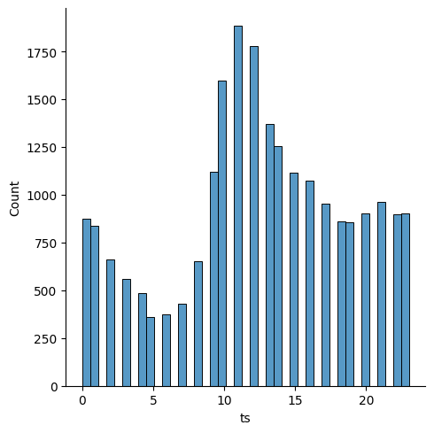
As shown with the previous analysis, 11 AM appears to be the peak listening hour of the year, the hour with the most streams throughout the months. Most of the streaming seems to be concentrated in the morning / early afternoon.
5. Conclusion
It is evident from the visuals that I started the year with my listening being highly concentrated in rap , with that share of my listening being reduced dramatically over the months as metal subgenres began to dominate my listening habits. You can observe this by looking at my top artists through out the months/seasons and from the Tableau dashboard’s stacked area chart.
The frequency at which rap was listened to is possibly higher than that of the metal subgenres as most of the rap genre streams are concentrated in the earlier parts of the year. While the metal subgenres have been streamed rather heavily since April or so.
Most of my listening was in Black Metal , with Departure Chandelier , Dissection, and Armagedda having the top albums in said genre. Albeit their placement in my list of top artists was not a perfect 1-to-1 image of my top three albums. As Unleashed (death metal), Immortal (black metal), and Darkthrone (black metal) were higher on the list of my top artists compared to Dissection. But my Dissection streams were largely contained to their 1st full-length album, the Somberlain. In contrast, my streaming habits for Unleashed, Immortal , and Darkthrone were spread out among more of their albums and EPs.
Thank you for taking the time to look at my post.